import statsmodels.formula.api as smf

model = smf.ols("outcome ~ treated * post", data=long).fit(
    cov_type="cluster", cov_kwds={"groups": long["unit_id"]}
)Week 8: Difference-in-Differences
Minimum wages and E-ZPass · PP5001 · Martinmas 2026
Class slides · Slides PDF · Notes PDF · Post-class exercise
Learning Objectives
By the end of this topic, you should be able to:
- Calculate a difference-in-differences estimate from four group means and represent its counterfactual graphically.
- Explain parallel trends in terms of untreated potential outcomes and derive the average treatment effect on the treated under that assumption.
- Connect the four means to the coefficients of a regression with group, period, and interaction terms.
- Assess a policy comparison using evidence about timing, group composition, spillovers, and other changes affecting the outcome.
- Estimate a basic DiD in Python and interpret its magnitude and uncertainty.
Before class
Read these notes and Card and Krueger (1994) and Currie and Walker (2011), available in Moodle. The first paper evaluates a minimum-wage increase using restaurants in two states. The second studies electronic toll collection and infant health using distance from toll plazas. Prepare to explain the policy, data, identification strategy, and results in each case.
Textbook references
Use the books to support your reading of the notes. You do not need to read all four accounts.
- The Effect: Chapter 18, Difference-in-Differences, especially the basic design and regression interpretation.
- Causal Inference: The Remix: Chapter 9, Difference-in-Differences Fundamentals.
- Mastering ’Metrics: Chapter 5, Differences-in-Differences. Companion resources and Mastering Econometrics videos at MRU.
- Mostly Harmless Econometrics — advanced reading: Chapter 5, Parallel Worlds: Fixed Effects, Differences-in-Differences, and Panel Data.
The Evaluation Problem
A policy begins at a particular time in a particular place. We observe outcomes before and after its introduction.
The before–after change combines:
- The effect of the policy.
- The change that would have occurred even without the policy.
We need a comparison that tells us about that second component.
For example, employment might fall after a minimum-wage increase because the policy reduced labour demand, because the economy entered a recession, or because both happened. Equally, a beneficial policy may be followed by a deterioration in outcomes if other conditions worsen sufficiently. The direction of the observed change alone does not identify the effect.
This is the same missing-counterfactual problem we have encountered throughout the module. Here, we observe the treated group at an earlier date. Its earlier outcome is useful, but time itself brings changes that we must account for.
Before and After
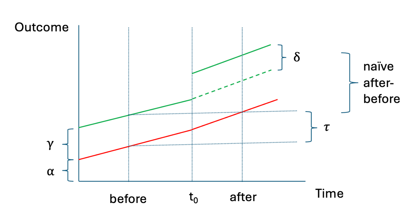
The graph distinguishes the observed post-policy outcome from the outcome that would have occurred without the intervention. A comparison with the pre-policy level attributes the entire change to treatment. To isolate the policy effect, we must also allow for the underlying change over time.
The Basic DiD Idea
Use the change in the control group to estimate the change the treated group would have experienced without treatment.
\widehat\delta_{DiD}= \left(\bar Y_{T,post}-\bar Y_{T,pre}\right) -\left(\bar Y_{C,post}-\bar Y_{C,pre}\right).
Taking each group’s change removes its fixed level. Subtracting the control group’s change removes the common change over time.
The subscripts T and C label the treatment and control groups. “Pre” and “post” label the two periods. Each bar denotes the sample mean in one of the four cells.
We can also subtract the treatment–control difference before the policy from the treatment–control difference after the policy. Rearranging the same four terms gives the same answer. Both calculations ask how the gap between the groups changed.
The 2×2 Parameterization
| Group | Before | After | Change |
|---|---|---|---|
| Treatment | \alpha+\gamma | \alpha+\gamma+\tau+\delta | \tau+\delta |
| Control | \alpha | \alpha+\tau | \tau |
| Treatment minus control | \gamma | \gamma+\delta | \delta |
\alpha: control-group baseline. \gamma: initial group difference.
\tau: common time change. \delta: the additional change in the treated group.
Start in the control group’s pre-policy cell. Its mean is \alpha. Moving to the treatment group adds \gamma. Moving to the post period adds \tau. The treatment group in the post period has one further component, \delta.
This parameterization can describe any four cell means. Interpreting \delta as a causal effect requires an assumption about how the treated group’s outcome would have changed without the policy. We will state that assumption explicitly below.
The Parameters in the Graph
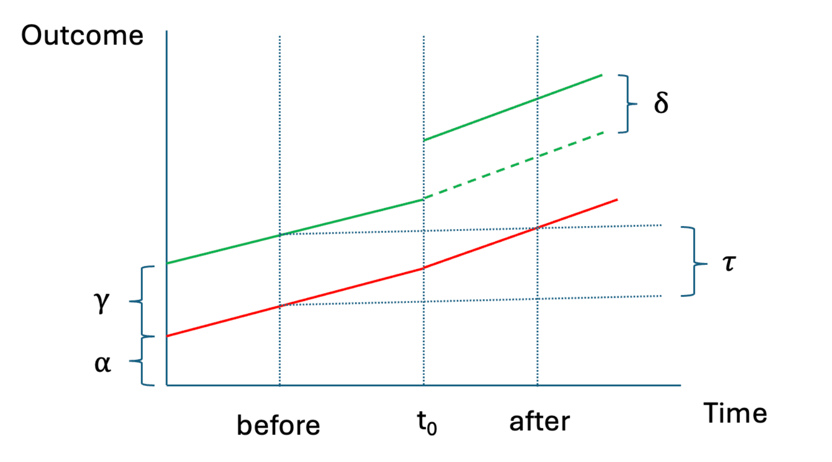
The original graph labels the common change \tau, the initial group difference \gamma, and the treatment effect \delta. The dashed continuation of the treated group’s path represents its counterfactual. The vertical gap between that path and the observed treated outcome after the policy is the effect of interest.
Regression Representation
Let T_i=1 identify membership in the treatment group and Post_t=1 identify the post-policy period.
Y_{it}=\alpha+\gamma T_i+\tau Post_t +\delta\left(T_i\times Post_t\right)+u_{it}.
- T_i allows the groups to have different initial levels.
- Post_t allows for the common time change.
- T_i\times Post_t equals one only for treated observations after the policy.
The individual or unit is indexed by i and time by t. In the restaurant example, i identifies a restaurant. In this basic design, group membership is fixed, while actual treatment exposure is D_{it}=T_i\times Post_t.
We use \tau consistently with the original graph. In the exercise’s generic coefficient notation, \beta_0=\alpha, \beta_1=\gamma, \beta_2=\tau, and \beta_3=\delta.
Why the Interaction Coefficient Is DiD
With an intercept and these three indicators, OLS fits all four cell means:
\begin{aligned} \hat\alpha&=\bar Y_{C,pre},\\ \hat\gamma&=\bar Y_{T,pre}-\bar Y_{C,pre},\\ \hat\tau&=\bar Y_{C,post}-\bar Y_{C,pre},\\ \hat\delta&=\bar Y_{T,post}-\hat\alpha-\hat\gamma-\hat\tau. \end{aligned}
Substituting the first three expressions into the last gives the difference-in-differences estimator.
To see the last step explicitly,
\begin{aligned} \hat\delta &=\bar Y_{T,post}-\bar Y_{C,pre} -\left(\bar Y_{T,pre}-\bar Y_{C,pre}\right) -\left(\bar Y_{C,post}-\bar Y_{C,pre}\right)\\ &=\left(\bar Y_{T,post}-\bar Y_{T,pre}\right) -\left(\bar Y_{C,post}-\bar Y_{C,pre}\right). \end{aligned}
There are four regression parameters and four group–period cells, so the regression can fit each cell mean exactly. This equivalence applies to the unadjusted regression using the same observations and weights as the calculation of means. Adding covariates or changing the sample changes the comparison.
Potential Outcomes and the ATT
Let Y_{it}^1 and Y_{it}^0 denote outcomes with and without treatment.
The effect of interest is
ATT=E\left[Y_{i,post}^1-Y_{i,post}^0\mid T_i=1\right].
We observe Y_{i,post}^1 for the treatment group. Its mean untreated outcome after the policy is the missing counterfactual.
Assume no anticipation and no spillovers to the control group.
Group membership T_i and treatment exposure D_{it} play different roles. Members of the treatment group are untreated in the pre period and treated in the post period. The control group remains untreated in both periods.
We assume no anticipation: the policy does not affect the treatment group’s pre-policy outcome. We also need the policy to leave the control group’s outcomes unaffected, including through spillovers. As in earlier weeks, outcomes must correspond to a well-defined treatment and be measured comparably.
Parallel Trends
In the absence of treatment, the two groups would have experienced the same average change:
E\left[Y_{i,post}^0-Y_{i,pre}^0\mid T_i=1\right] = E\left[Y_{i,post}^0-Y_{i,pre}^0\mid T_i=0\right].
The groups may start at different levels. The assumption concerns their changes in untreated potential outcomes.
This is an assumption about a counterfactual after treatment starts. We can observe the control group’s untreated change. For the treatment group, we observe its pre-policy untreated outcome and its post-policy treated outcome. We cannot directly observe the untreated post-policy change on the left-hand side.
A convincing argument therefore needs knowledge of why the policy was adopted, why the comparison group is suitable, and what other events occurred. If several earlier periods are available, similar prior trends can support that argument. Their similarity cannot guarantee that the counterfactual trends would remain parallel after the policy starts.
Constructing the Counterfactual
Parallel trends implies
\begin{aligned} E\left[Y_{i,post}^0\mid T_i=1\right] ={}&E\left[Y_{i,pre}^0\mid T_i=1\right]\\ &+E\left[Y_{i,post}^0-Y_{i,pre}^0\mid T_i=0\right]. \end{aligned}
Treated group’s baseline + control group’s change = treated group’s counterfactual post-policy mean.
The assumption lets us fill in the missing cell. Begin at the treatment group’s observed baseline and add the change observed in the control group. This preserves the initial difference between the groups while applying a common untreated trend.
The counterfactual may rise or fall. A positive treatment effect means that the observed outcome exceeds this counterfactual, even if the treatment group’s observed outcome falls over time.
From the Counterfactual to the Effect
Substitute that counterfactual into the definition of the ATT:
\begin{aligned} ATT={}&E\left[Y_{i,post}\mid T_i=1\right] -E\left[Y_{i,pre}\mid T_i=1\right]\\ &-\left(E\left[Y_{i,post}\mid T_i=0\right] -E\left[Y_{i,pre}\mid T_i=0\right]\right). \end{aligned}
Use the analogy principle to replace the four population conditional means with their sample counterparts.
We can write these expectations using observed Y because of the treatment pattern and no-anticipation assumption: the treatment group reveals its treated outcome after the policy and its untreated outcome before it. The control group reveals untreated outcomes in both periods.
This derivation allows effects to differ across treated units. The basic DiD identifies their average post-policy effect under the stated assumptions. It does not require each restaurant or each mother to experience the same effect.
Different Underlying Trends
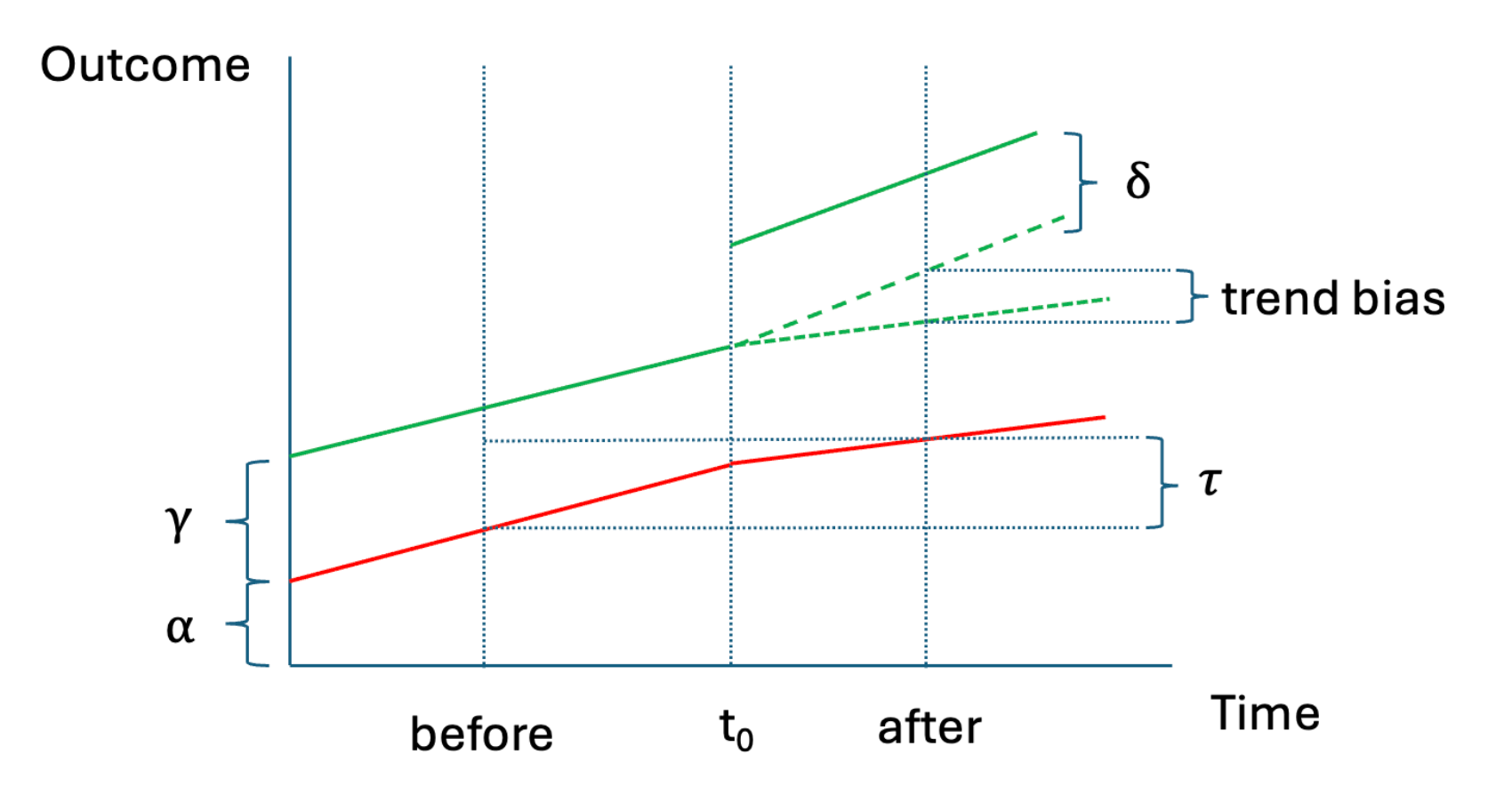
If the treatment group’s untreated outcome would have grown faster, the control group’s change understates its counterfactual growth. The DiD then attributes some of that extra growth to the policy. A slower untreated trend produces the opposite error.
More formally, the population DiD equals the ATT plus
E\left[Y_{i,post}^0-Y_{i,pre}^0\mid T_i=1\right] -E\left[Y_{i,post}^0-Y_{i,pre}^0\mid T_i=0\right].
Parallel trends sets this second component to zero. Increasing the number of observations can make the estimate more precise without removing a systematic difference in those untreated trends.
Card and Krueger: Policy, Data, and Identification
For discussion: What changed in New Jersey? Who was surveyed, when, and why is eastern Pennsylvania a plausible control group? State the identifying assumption in this setting.
New Jersey raised its minimum wage from $4.25 to $5.05 per hour on 1 April 1992. Pennsylvania’s minimum remained $4.25. Card and Krueger surveyed fast-food restaurants in February–March and again in November–December. The initial sample contained 410 restaurants.
Fast-food restaurants employ many low-wage workers, making the policy particularly relevant to them. Nearby Pennsylvania restaurants provide a comparison exposed to some of the same regional economic conditions. The causal argument still requires that their employment changes represent what New Jersey restaurants would have experienced without the increase.
The study followed existing restaurants. Its employment measure includes changes at restaurants that closed, but the design does not directly measure employment generated by new restaurant openings. Keep that scope in mind when making a policy recommendation.
Card and Krueger: Figure 1
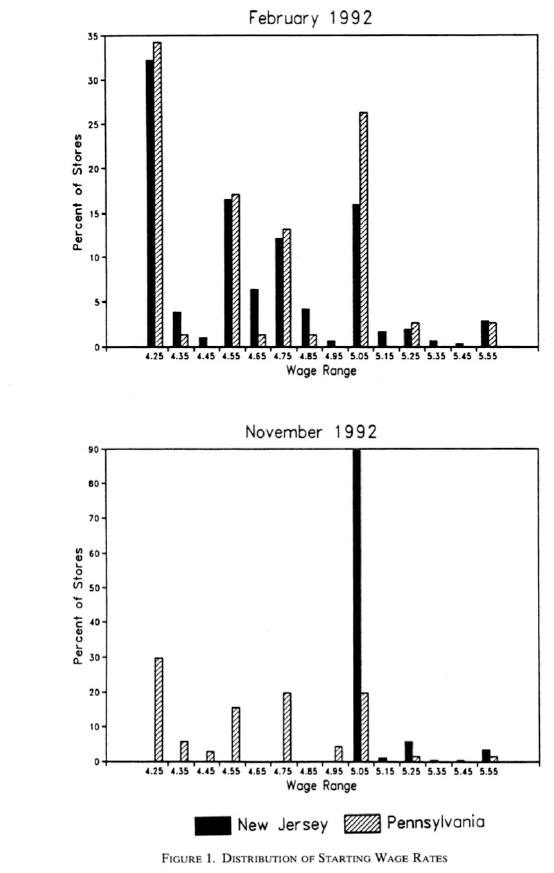
Card and Krueger (1994), Figure 1.
The distributions of starting wages show how the increase changed the wage floor in New Jersey relative to Pennsylvania. This provides evidence that the policy affected the price of labour faced by the sampled restaurants. The employment comparison then asks how employment responded.
Card and Krueger: Table 3
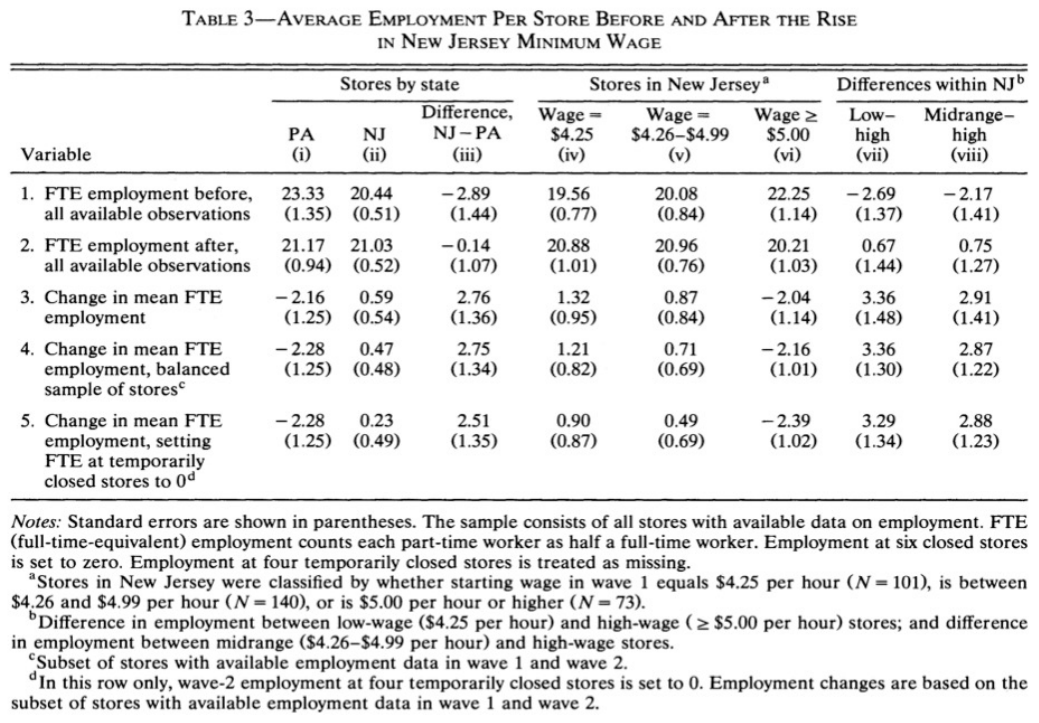
For discussion: Explain columns (i)–(iii), including the DiD. Why do rows 3 and 4 differ? What is a full-time-equivalent employee?
Full-time-equivalent employment counts managers and full-time employees at weight one and part-time employees at weight one-half. The unit is an equivalent full-time employee per restaurant.
Rows 1 and 2 report the available employment means in each wave. Row 3 differences those means. Row 4 uses restaurants with employment observed in both periods, holding the set of restaurants fixed. Missing employment information means these are slightly different comparisons. The distinction matters when translating a published table into code.
The post-class exercise reproduces these calculations. It then uses the balanced sample to show that the four-means calculation and the regression interaction coefficient agree. Permanently closed restaurants have zero post-period employment in the data, which is part of the policy-relevant outcome rather than a missing observation.
Covariates in the Levels Model
Let X_{ik} be pre-treatment characteristics held fixed across the two periods.
\begin{aligned} Y_{it}={}&\alpha+\gamma T_i+\tau Post_t +\delta\left(T_i\times Post_t\right)\\ &+\sum_{k=1}^{K}\beta_k X_{ik} +\sum_{k=1}^{K}\theta_k\left(X_{ik}\times Post_t\right)+u_{it}. \end{aligned}
- \beta_k allows baseline outcomes to differ with X_{ik}.
- \theta_k allows the change over time to differ with X_{ik}.
- \delta is the additional change associated with treatment, conditional on these characteristics.
The original parameters keep their meanings: \alpha is the control-group baseline when the covariates equal zero, \gamma is the initial group difference conditional on the covariates, \tau is the control-group time change at those reference values, and \delta is the treatment-group additional change. The new coefficients are \beta_k for baseline covariate differences and \theta_k for covariate-specific changes.
For example, restaurants from different chains may start with different employment levels and may experience different employment changes. The terms involving \beta_k allow the first pattern. The interactions with Post_t, with coefficients \theta_k, allow the second.
For a causal interpretation, we need a credible parallel-trends argument conditional on the pre-treatment characteristics, appropriate overlap, and a suitable regression specification. In this additive model, a common \delta represents the conditional treatment effect. With heterogeneous effects, an adjusted OLS coefficient need not equal the overall ATT without further restrictions or appropriate averaging.
From Levels to Differences with Covariates
For the same unit, subtract the pre-period equation from the post-period equation:
\Delta Y_i=\tau+\delta T_i +\sum_{k=1}^{K}\theta_k X_{ik}+\Delta u_i.
- \alpha, \gamma T_i, and \sum_{k=1}^{K}\beta_kX_{ik} cancel.
- \tau, \delta, and \theta_k retain exactly the same meanings.
- Card–Krueger Table 4 uses employment changes as the outcome, with chain and ownership indicators entered directly as controls.
Here \Delta Y_i=Y_{i,post}-Y_{i,pre} and \Delta u_i=u_{i,post}-u_{i,pre}. Before the policy, both Post_t and T_i\times Post_t are zero. After the policy, Post_t=1 and T_i\times Post_t=T_i. Since the characteristics are held fixed, their baseline contributions cancel while their post-period interactions leave \theta_k X_{ik}.
Thus the covariate coefficients in the change regression are the \theta_k coefficients from the levels model. Chain and ownership indicators allow different types of restaurants to experience different employment changes.
Card and Krueger estimate the change regression directly. The preceding levels equation shows how that specification can be represented with period interactions. Adding the fixed characteristics to a levels regression only as main effects would allow baseline differences but would not allow these covariate-specific changes.
For a balanced two-period sample with these same fixed covariates and all the displayed interactions, OLS in levels and OLS in changes give the same treatment-effect point estimate. Their standard errors must account for the different representations of repeated observations and may use different finite-sample corrections.
Card and Krueger: Table 4
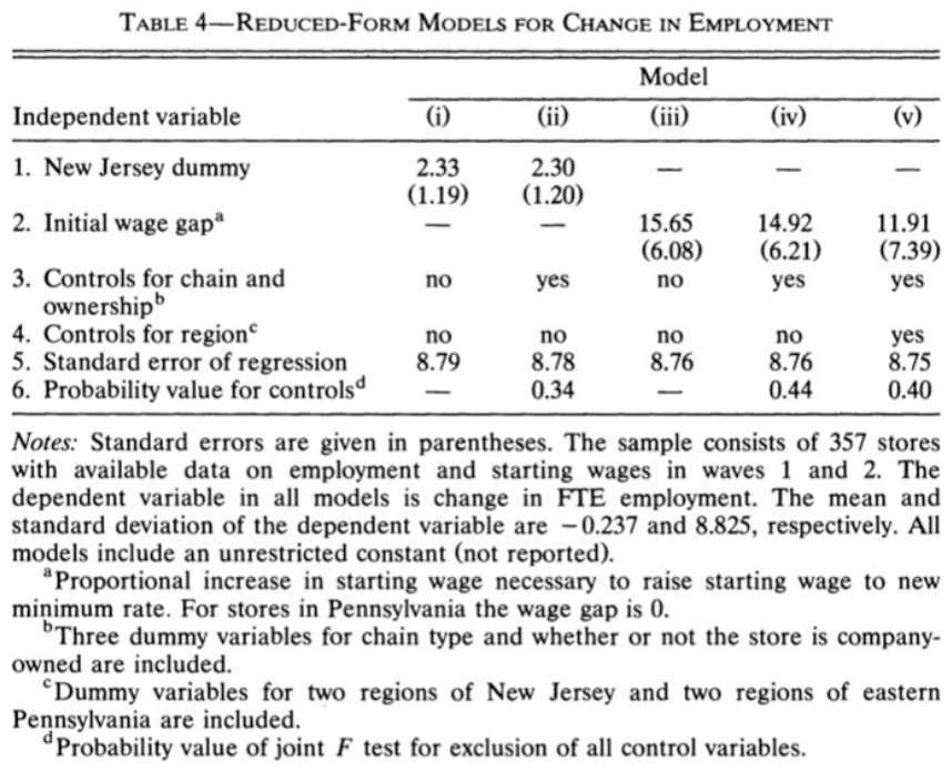
For discussion: Compare columns (i) and (ii). Why might chain and ownership matter? Separate the change in sample from the effect of adding controls.
The dependent variable is the change in employment. Column (i) regresses that change on the New Jersey indicator and an intercept. Column (ii) adds indicators for chain and company ownership. These allow average employment changes to differ across those types of restaurants.
The sample is smaller than the balanced sample used in Table 3. The paper restricts the subsequent regression analysis to restaurants with the employment and wage information needed for those comparisons. Consequently, a difference between Table 3 and Table 4, column (i), can arise from changing the sample. The comparison between columns (i) and (ii) isolates the addition of the chain and ownership controls on the same sample.
Both columns give positive New Jersey estimates. Adding controls changes the magnitude only modestly. This is useful evidence about those measured differences, while the causal interpretation still depends on the comparison group’s counterfactual employment trend.
Currie and Walker: The Policy
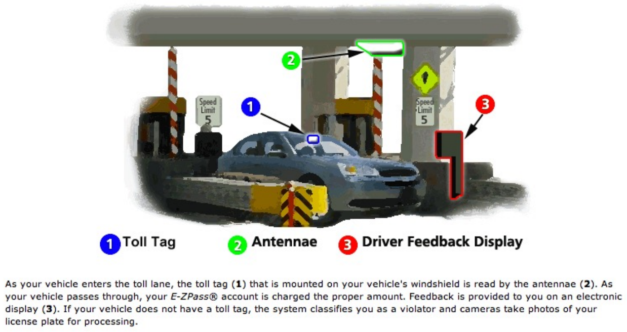
E-ZPass allows electronic toll collection, reducing stops and queues at toll plazas. The study asks whether the resulting changes improve infant health nearby.
The mechanism connects transport policy to local exposure: less queuing and idling may reduce vehicle emissions near a toll plaza. Pregnancy provides a period during which changes in exposure could affect birth outcomes. This gives us a second application of the same comparison of changes, with a very different policy and outcome.
Currie and Walker: Data and Identification
For discussion: Define the treatment and control groups, the timing of treatment, and the birth outcomes. Why compare mothers near the same road network? State parallel trends for this design.
The researchers link geocoded birth records in New Jersey and Pennsylvania to toll-plaza locations and E-ZPass adoption dates. Their central comparison uses mothers within 2 km of a toll plaza and mothers between 2 and 10 km away, with the latter also living within 3 km of a major highway.
The control group helps account for changes affecting mothers living near major roads. The assumption is that birth outcomes near toll plazas would have changed like those in the comparison areas without E-ZPass. The published analysis includes multiple locations and adoption dates. We use the near-versus-far, before-versus-after contrast to understand its logic here. The fuller treatment of timing and multiple periods follows in the next sessions.
Where Are the Comparisons Made?
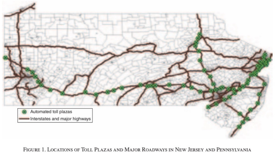
Currie and Walker (2011), Figure 1.
The map places the treatment and comparison areas in their regional setting. Proximity makes some shared economic and environmental changes plausible, but it also raises questions about spillovers. For example, changes in traffic patterns could affect nearby comparison areas as well as the area immediately around a toll plaza.
Currie and Walker: Table 3
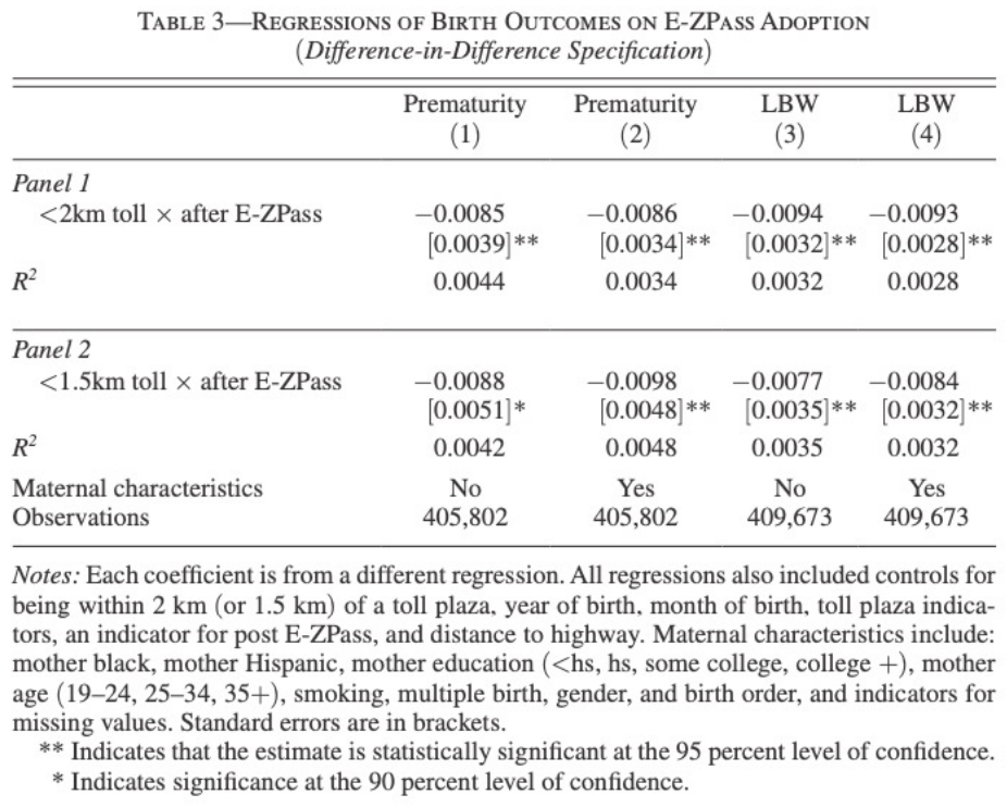
For discussion: Interpret the prematurity and low-birth-weight estimates in Panel 1. Distinguish percentage points from percentages. How do the estimates change when maternal characteristics are included?
Prematurity and low birth weight are binary outcomes. A coefficient of -0.009 in a linear probability model represents a decline of 0.9 percentage points. A percentage reduction requires dividing that change by a relevant baseline probability. Always state the baseline used.
Panel 1 uses the 2 km treatment radius. The columns compare specifications with and without maternal characteristics. Panel 2 changes the treatment radius to 1.5 km. This comparison helps assess how sensitive the estimates are to the definition of local exposure.
For the class discussion, distinguish three questions: the direction and size of the estimate, its uncertainty, and the assumptions needed to interpret it causally. A precise coefficient addresses the second question but cannot settle the third.
Currie and Walker: Table 2
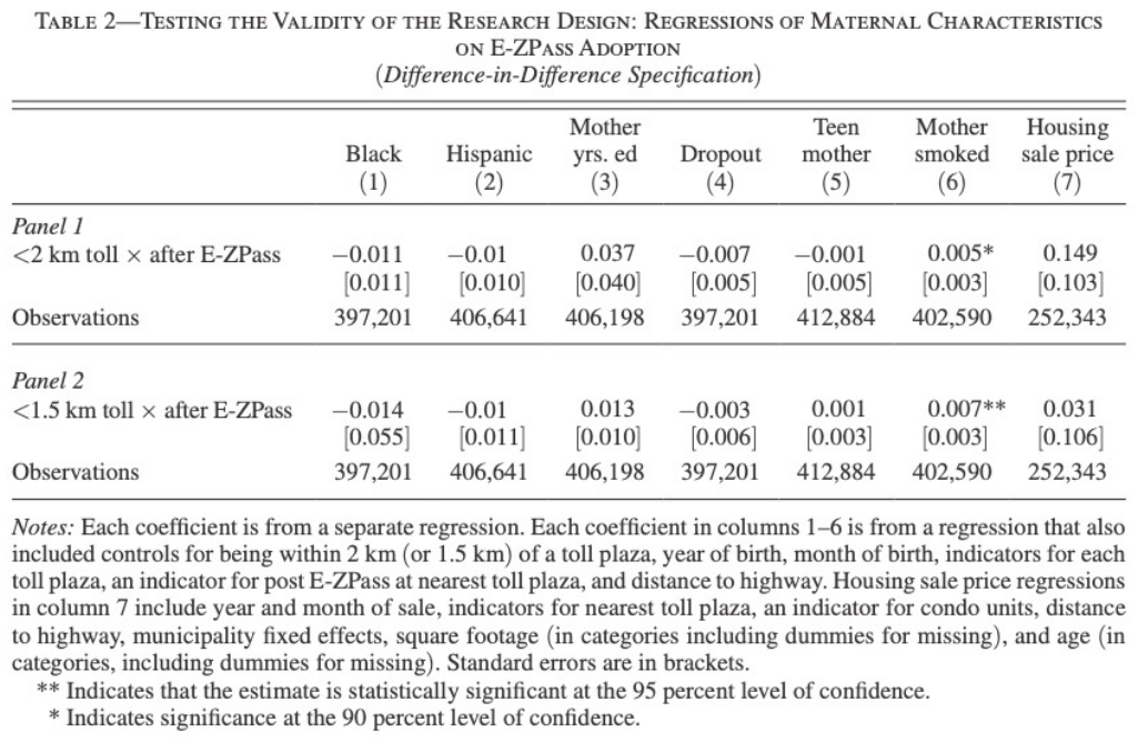
For discussion: Could changes in who lives near toll plazas explain the health results? What does this table tell us, and what uncertainty remains?
The authors apply the comparison of changes to maternal characteristics. If E-ZPass led different families to move into areas near toll plazas, changes in infant health could partly reflect the changing composition of births observed there.
Small and imprecise changes in measured characteristics are reassuring to the extent that they rule out substantively important changes. They still leave room for changes in unmeasured characteristics. Consider the estimates and their uncertainty rather than treating a set of insignificant coefficients as proof of comparability.
Housing-market responses offer another way to investigate sorting. The timing matters: a policy could have little immediate effect on residential composition but affect it over a longer period.
Currie and Walker: Table 7
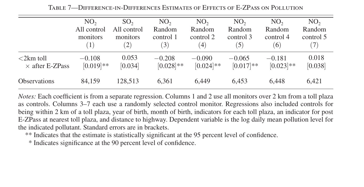
For discussion: Compare the two pollutants. How does this evidence support the proposed mechanism? What does having only one monitor near a toll plaza imply?
The dependent variables are log daily mean pollutant levels. Column (1)’s coefficient of -0.108 corresponds approximately to a 10.8% reduction in nitrogen dioxide. The exact proportional change is \exp\left(-0.108\right)-1, or about a 10.2% reduction. The sulfur dioxide comparison is useful because traffic is a much more important source of the first pollutant.
There is only one monitor within 2 km of a toll plaza. Many observations over days provide information about that location, but they do not create many independently treated locations. This limits the strength and generality of the pollution evidence.
The pollution analysis supports a mechanism linking E-ZPass to health. Estimating the causal effect of pollution itself would additionally require an appropriate first stage, an exclusion restriction ruling out other channels from E-ZPass to health, and a compatible population and exposure measure.
What Can Threaten the Comparison?
- Different underlying trends: a local shock changes the treated group’s outcome independently of the policy.
- Anticipation: behaviour changes before the designated treatment date.
- Spillovers: the policy affects the control group.
- Composition: the people or establishments observed change over time.
In Card–Krueger, ask whether regional economic developments could have affected employment differently across states and whether restaurants adjusted before April. In Currie–Walker, ask whether traffic was displaced and whether the composition of mothers changed.
Treating closures correctly illustrates why composition requires care. Zero employment at a closed restaurant is a meaningful outcome. Dropping closed restaurants would change the question to employment among survivors, whose survival may itself have been affected by treatment.
Controls and Evidence on Trends
Use institutional knowledge to motivate the comparison. Examine earlier trends when the data allow it.
Choose controls with a clear role in the design. Variables affected by the policy may remove part of the effect we want to estimate or introduce selection.
Adding controls can account for measured differences in how outcomes would otherwise change. It requires a corresponding argument that the remaining untreated trends are comparable conditional on those controls. Similar baseline levels alone cannot supply that argument.
With only one pre-policy period, we cannot compare pre-policy slopes. With several, plots can reveal differences before treatment and help identify anticipation. A failure to reject a pre-trend test may also reflect limited precision. Event studies will give us a systematic way to examine these patterns in the next session.
Uncertainty and the Level of Treatment
Many individuals can share the same policy and the same shocks.
- Restaurants share state-level economic conditions.
- Repeated observations on a restaurant can have correlated disturbances.
- Daily observations at a monitor can share persistent local conditions.
The number of observations is different from the number of independent policy comparisons.
Heteroskedasticity-consistent standard errors allow the disturbance variance to differ across observations but ordinarily retain independence across observations. Clustered standard errors also allow disturbances to be correlated within a specified group.
In the exercise, clustering by restaurant accounts for the two observations from each restaurant. It does not account for shocks shared by different restaurants in the same state. With only two states, usual methods that rely on many independent state clusters cannot be justified simply by requesting state-clustered standard errors. The reported uncertainty should therefore be read alongside the institutional argument and the limited number of policy comparisons.
From Four Means to Python
For data with one row per unit and period:
treated * post includes both indicators and their interaction. The interaction coefficient is the unadjusted DiD.
Here treated identifies the treatment group in both periods and post identifies the later period in both groups. The variable unit_id links repeated observations on the same unit. Replace these generic names with the actual columns in your data.
The post-class notebook supplies the import and reshaping code for Card–Krueger. You calculate the means, plot the counterfactual, and interpret the coefficients. Using the same sample at each step is essential for verifying the equivalence.
Changes as the Dependent Variable
With the same units observed twice, subtract each unit’s pre-period equation from its post-period equation:
\Delta Y_i=\tau+\delta T_i+\Delta u_i.
The intercept is the control group’s average change. The coefficient on T_i is the difference between the groups’ changes.
The constant \alpha and the time-invariant group component \gamma T_i cancel. The post indicator changes from zero to one. Treatment exposure also changes from zero to one for the treatment group, while remaining zero for controls.
This gives a second regression implementation of the same 2×2 comparison. Use the same balanced sample to verify equality of the point estimates. Standard-error corrections can differ slightly between implementations, so exact equality of coefficients does not imply numerical identity of every reported statistic.
What a Credible DiD Design Needs
- Clear policy timing and a well-defined outcome.
- A plausible comparison group and an explicit parallel-trends argument.
- Evidence on other changes, anticipation, spillovers, and composition.
- Uncertainty appropriate to the available independent comparisons.
The control group supplies the change used to construct the treated group’s counterfactual.
References
Card, D., and A. B. Krueger (1994). Minimum Wages and Employment: A Case Study of the Fast-Food Industry in New Jersey and Pennsylvania. American Economic Review, 84(4), 772–793.
Currie, J., and R. Walker (2011). Traffic Congestion and Infant Health: Evidence from E-ZPass. American Economic Journal: Applied Economics, 3(1), 65–90.
Angrist, J. D., and J.-S. Pischke (2015). Mastering ’Metrics: The Path from Cause to Effect. Chapter 5.
Angrist, J. D., and J.-S. Pischke (2009). Mostly Harmless Econometrics: An Empiricist’s Companion. Chapter 5. Advanced reading.
Cunningham, S. Causal Inference: The Remix. Chapter 9, linked above.
Huntington-Klein, N. The Effect: An Introduction to Research Design and Causality. Chapter 18, linked above.