Difference-in-Differences
PP5001 · Week 8 · Martinmas 2026
Professor David A. Jaeger
The Evaluation Problem
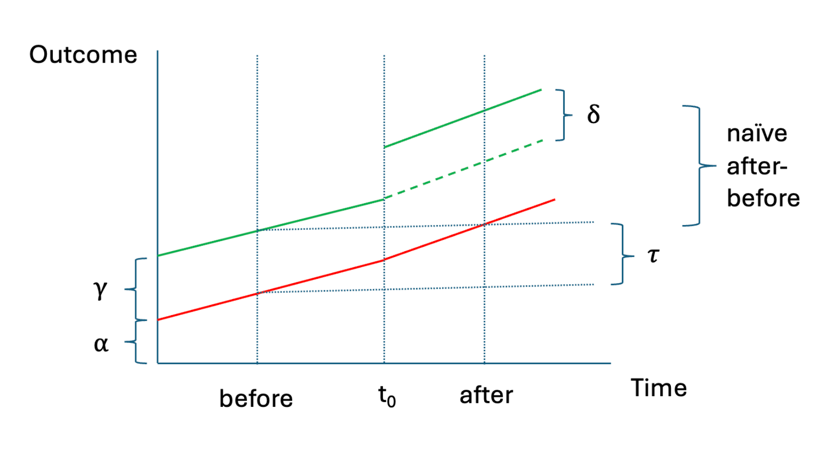
A policy begins at a particular time in a particular place. We observe outcomes before and after its introduction.
The before–after change combines:
- The effect of the policy.
- The change that would have occurred even without the policy.
We need a comparison that tells us about that second component.
Before and After
![Before–after comparison from the original lecture slides.]()
The Basic DiD Idea
Use the change in the control group to estimate the change the treated group would have experienced without treatment.
\widehat\delta_{DiD}=
\left(\bar Y_{T,post}-\bar Y_{T,pre}\right)
-\left(\bar Y_{C,post}-\bar Y_{C,pre}\right).
Taking each group’s change removes its fixed level. Subtracting the control group’s change removes the common change over time.
The 2×2 Parameterization
| Treatment |
\alpha+\gamma |
\alpha+\gamma+\tau+\delta |
\tau+\delta |
| Control |
\alpha |
\alpha+\tau |
\tau |
| Treatment minus control |
\gamma |
\gamma+\delta |
\delta |
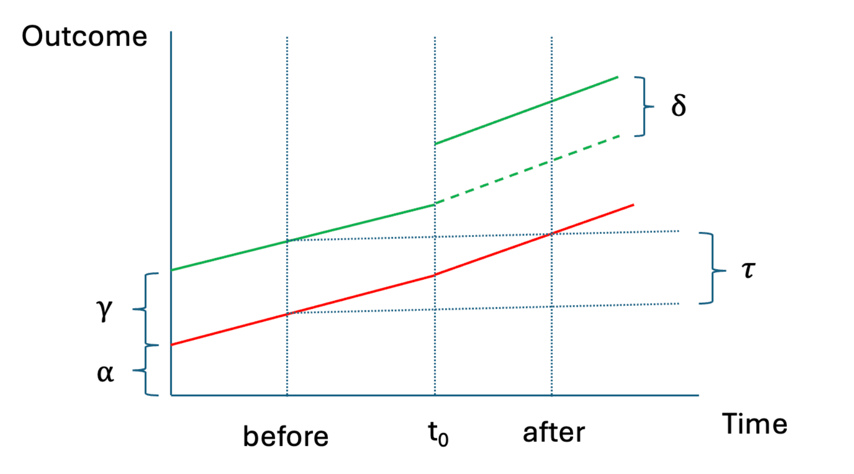
\alpha: control-group baseline. \gamma: initial group difference.
\tau: common time change. \delta: the additional change in the treated group.
The Parameters in the Graph
![DiD parameterization from the original lecture slides.]()
Regression Representation
Let T_i=1 identify membership in the treatment group and Post_t=1 identify the post-policy period.
Y_{it}=\alpha+\gamma T_i+\tau Post_t
+\delta\left(T_i\times Post_t\right)+u_{it}.
- T_i allows the groups to have different initial levels.
- Post_t allows for the common time change.
- T_i\times Post_t equals one only for treated observations after the policy.
Why the Interaction Coefficient Is DiD
With an intercept and these three indicators, OLS fits all four cell means:
\begin{aligned}
\hat\alpha&=\bar Y_{C,pre},\\
\hat\gamma&=\bar Y_{T,pre}-\bar Y_{C,pre},\\
\hat\tau&=\bar Y_{C,post}-\bar Y_{C,pre},\\
\hat\delta&=\bar Y_{T,post}-\hat\alpha-\hat\gamma-\hat\tau.
\end{aligned}
Substituting the first three expressions into the last gives the difference-in-differences estimator.
Potential Outcomes and the ATT
Let Y_{it}^1 and Y_{it}^0 denote outcomes with and without treatment.
The effect of interest is
ATT=E\left[Y_{i,post}^1-Y_{i,post}^0\mid T_i=1\right].
We observe Y_{i,post}^1 for the treatment group. Its mean untreated outcome after the policy is the missing counterfactual.
Assume no anticipation and no spillovers to the control group.
Parallel Trends
In the absence of treatment, the two groups would have experienced the same average change:
E\left[Y_{i,post}^0-Y_{i,pre}^0\mid T_i=1\right]
=
E\left[Y_{i,post}^0-Y_{i,pre}^0\mid T_i=0\right].
The groups may start at different levels. The assumption concerns their changes in untreated potential outcomes.
Constructing the Counterfactual
Parallel trends implies
\begin{aligned}
E\left[Y_{i,post}^0\mid T_i=1\right]
={}&E\left[Y_{i,pre}^0\mid T_i=1\right]\\
&+E\left[Y_{i,post}^0-Y_{i,pre}^0\mid T_i=0\right].
\end{aligned}
Treated group’s baseline + control group’s change = treated group’s counterfactual post-policy mean.
From the Counterfactual to the Effect
Substitute that counterfactual into the definition of the ATT:
\begin{aligned}
ATT={}&E\left[Y_{i,post}\mid T_i=1\right]
-E\left[Y_{i,pre}\mid T_i=1\right]\\
&-\left(E\left[Y_{i,post}\mid T_i=0\right]
-E\left[Y_{i,pre}\mid T_i=0\right]\right).
\end{aligned}
Use the analogy principle to replace the four population conditional means with their sample counterparts.
Different Underlying Trends
![Trend bias from the original lecture slides.]()
Card and Krueger: Policy, Data, and Identification
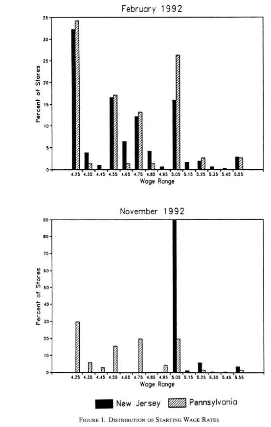
For discussion: What changed in New Jersey? Who was surveyed, when, and why is eastern Pennsylvania a plausible control group? State the identifying assumption in this setting.
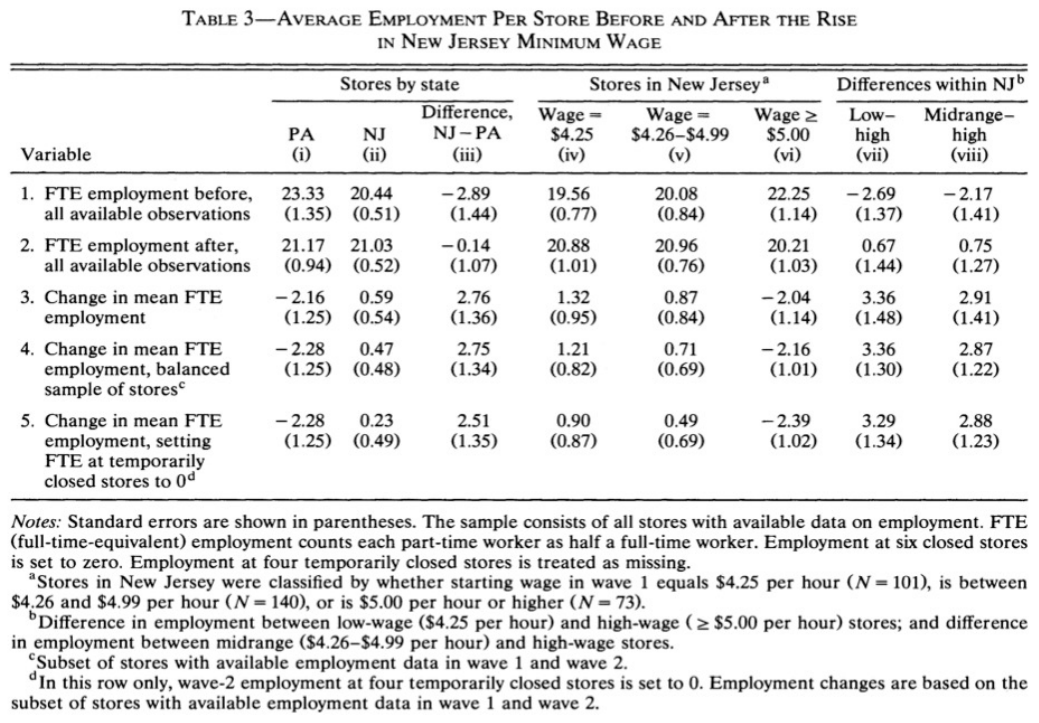
Card and Krueger: Table 3
![Card and Krueger Table 3, average employment before and after.]()
For discussion: Explain columns (i)–(iii), including the DiD. Why do rows 3 and 4 differ? What is a full-time-equivalent employee?
Covariates in the Levels Model
Let X_{ik} be pre-treatment characteristics held fixed across the two periods.
\begin{aligned}
Y_{it}={}&\alpha+\gamma T_i+\tau Post_t
+\delta\left(T_i\times Post_t\right)\\
&+\sum_{k=1}^{K}\beta_k X_{ik}
+\sum_{k=1}^{K}\theta_k\left(X_{ik}\times Post_t\right)+u_{it}.
\end{aligned}
- \beta_k allows baseline outcomes to differ with X_{ik}.
- \theta_k allows the change over time to differ with X_{ik}.
- \delta is the additional change associated with treatment, conditional on these characteristics.
From Levels to Differences with Covariates
For the same unit, subtract the pre-period equation from the post-period equation:
\Delta Y_i=\tau+\delta T_i
+\sum_{k=1}^{K}\theta_k X_{ik}+\Delta u_i.
- \alpha, \gamma T_i, and \sum_{k=1}^{K}\beta_kX_{ik} cancel.
- \tau, \delta, and \theta_k retain exactly the same meanings.
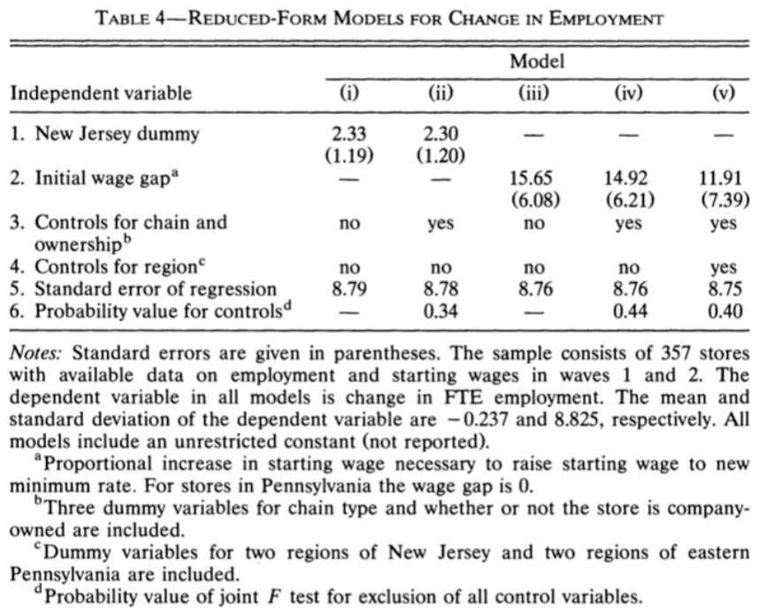
- Card–Krueger Table 4 uses employment changes as the outcome, with chain and ownership indicators entered directly as controls.
Card and Krueger: Table 4
![Card and Krueger Table 4, regressions for the employment change.]()
For discussion: Compare columns (i) and (ii). Why might chain and ownership matter? Separate the change in sample from the effect of adding controls.
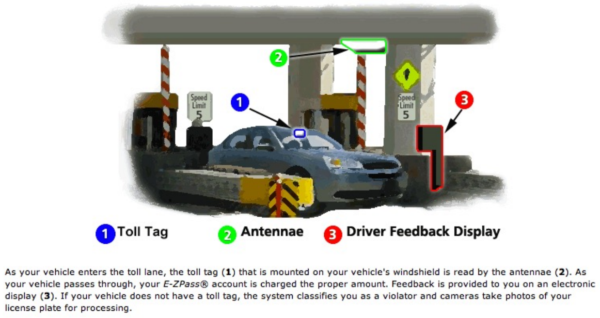
Currie and Walker: The Policy
![Electronic toll collection illustration from the original lecture materials.]()
E-ZPass allows electronic toll collection, reducing stops and queues at toll plazas. The study asks whether the resulting changes improve infant health nearby.
Currie and Walker: Data and Identification
For discussion: Define the treatment and control groups, the timing of treatment, and the birth outcomes. Why compare mothers near the same road network? State parallel trends for this design.
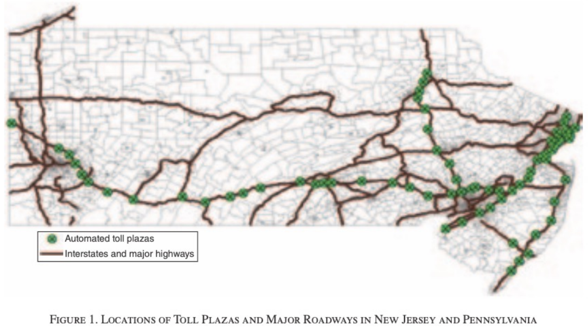
Where Are the Comparisons Made?
![Currie and Walker map of toll plazas and major roads.]()
Currie and Walker (2011), Figure 1.
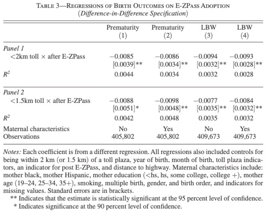
Currie and Walker: Table 3
![Currie and Walker Table 3, infant-health outcomes.]()
For discussion: Interpret the prematurity and low-birth-weight estimates in Panel 1. Distinguish percentage points from percentages. How do the estimates change when maternal characteristics are included?
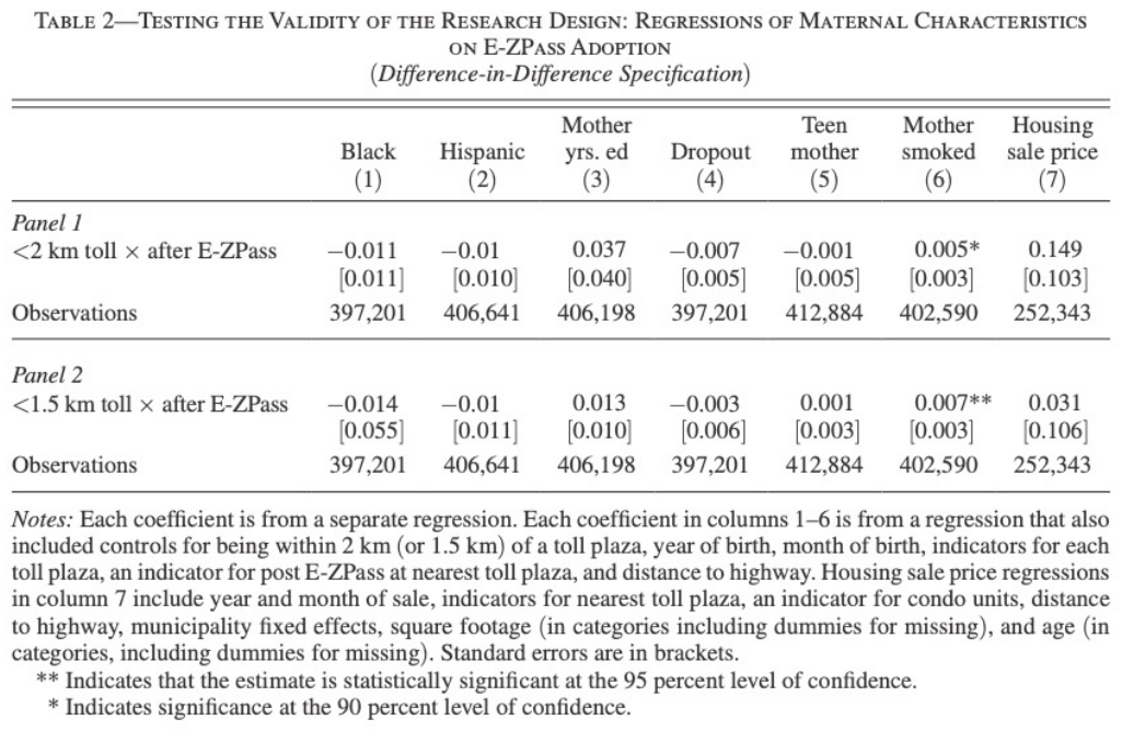
Currie and Walker: Table 2
![Currie and Walker Table 2, maternal characteristics.]()
For discussion: Could changes in who lives near toll plazas explain the health results? What does this table tell us, and what uncertainty remains?
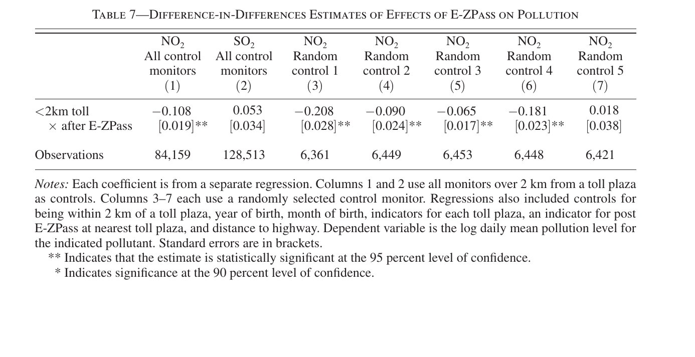
Currie and Walker: Table 7
![Currie and Walker Table 7, effects on air pollution.]()
For discussion: Compare the two pollutants. How does this evidence support the proposed mechanism? What does having only one monitor near a toll plaza imply?
What Can Threaten the Comparison?
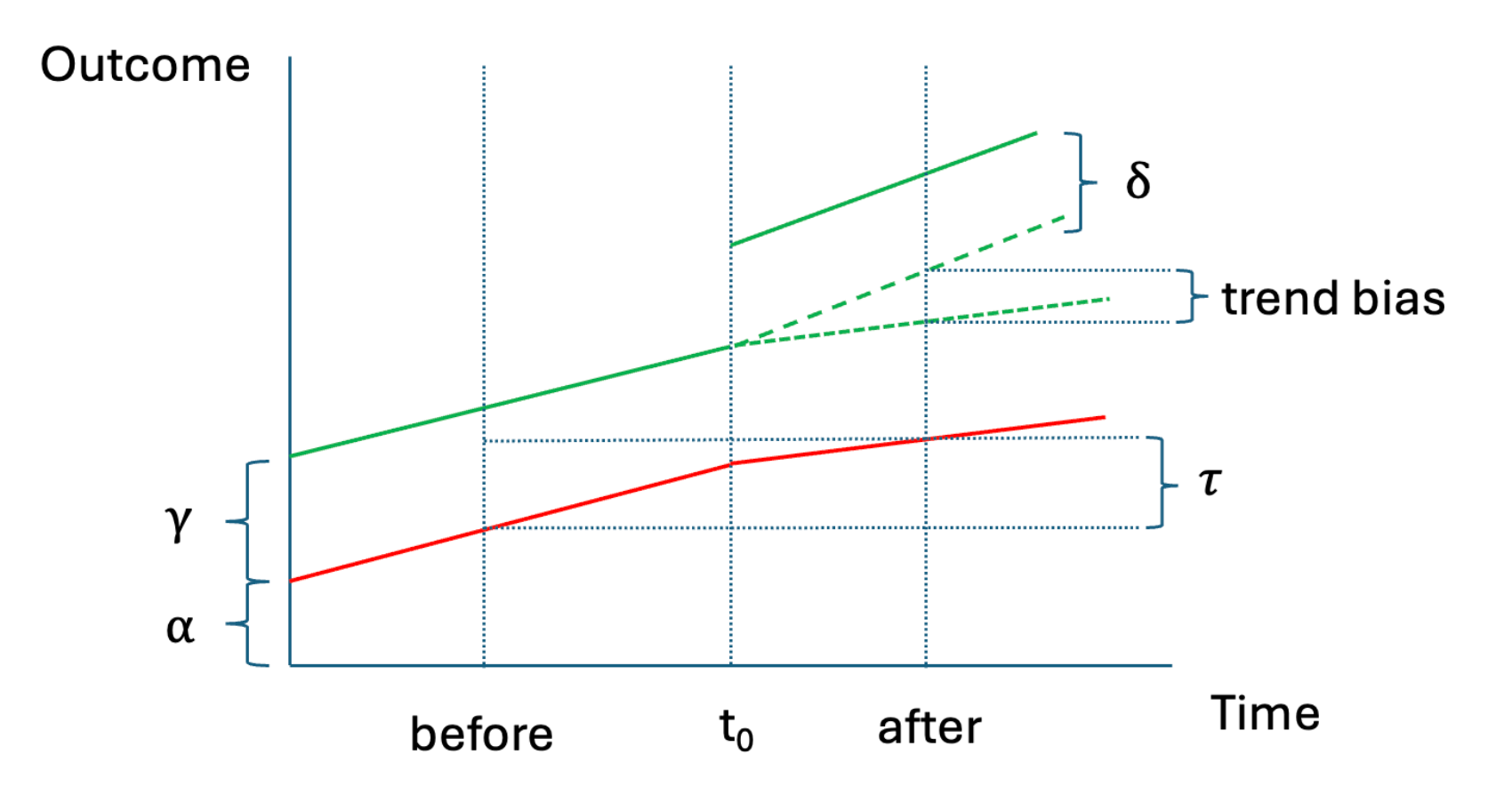
- Different underlying trends: a local shock changes the treated group’s outcome independently of the policy.
- Anticipation: behaviour changes before the designated treatment date.
- Spillovers: the policy affects the control group.
- Composition: the people or establishments observed change over time.
Controls and Evidence on Trends
Use institutional knowledge to motivate the comparison. Examine earlier trends when the data allow it.
Choose controls with a clear role in the design. Variables affected by the policy may remove part of the effect we want to estimate or introduce selection.
Uncertainty and the Level of Treatment
Many individuals can share the same policy and the same shocks.
- Restaurants share state-level economic conditions.
- Repeated observations on a restaurant can have correlated disturbances.
- Daily observations at a monitor can share persistent local conditions.
The number of observations is different from the number of independent policy comparisons.
Changes as the Dependent Variable
With the same units observed twice, subtract each unit’s pre-period equation from its post-period equation:
\Delta Y_i=\tau+\delta T_i+\Delta u_i.
The intercept is the control group’s average change. The coefficient on T_i is the difference between the groups’ changes.
What a Credible DiD Design Needs
- Clear policy timing and a well-defined outcome.
- A plausible comparison group and an explicit parallel-trends argument.
- Evidence on other changes, anticipation, spillovers, and composition.
- Uncertainty appropriate to the available independent comparisons.
The control group supplies the change used to construct the treated group’s counterfactual.