import numpy as np
import pandas as pd
import matplotlib.pyplot as plt
import statsmodels.formula.api as smf
import rdrobust as rd
import rddensity as density

# A seed keeps the sample unchanged when we run the code again.
rng = np.random.default_rng(2026)
n = 20000
original_score = rng.uniform(-2, 2, n)
ability = rng.normal(0, 1, n)
outcome_noise = rng.normal(0, 1, n)

# The score determines eligibility. The true treatment effect is 2.
treatment_before = (original_score >= 0).astype(int)
outcome_without_treatment = 10 + 0.5 * original_score + 2 * ability + outcome_noise
outcome_before = outcome_without_treatment + 2 * treatment_beforeWeek 7: Regression Discontinuity Designs
Elections and class size · PP5001 · Martinmas 2026
Class slides · Slides PDF · Notes PDF · Quarto source · Python simulation · Post-class exercise
Learning Objectives
By the end of this topic, you should be able to:
- Distinguish sharp and fuzzy regression discontinuity designs and explain how continuity of potential-outcome means identifies an effect at the cutoff.
- Explain how bandwidth and kernel choices determine which observations contribute to a local regression estimate.
- Assess the credibility of an RD design using institutional knowledge, covariate evidence, and a test for a discontinuity in the running-variable density.
- Estimate and interpret a sharp RD effect, explain how IV estimates a fuzzy RD effect, and assess the policy relevance of these local effects.
Before class
Read these notes and the four empirical papers: Lee (2008), Meyersson (2014), Angrist and Lavy (1999), and Angrist, Lavy, Leder-Luis and Shany (2019). The papers are on Moodle. Lee motivates the design. We use Meyersson to examine sharp RD and the two class-size papers to examine fuzzy RD and the credibility of the assignment mechanism.
Textbook references
- The Effect: Chapter 20, Regression Discontinuity.
- Causal Inference: The Remix: Chapter 6, Regression Discontinuity.
- Mastering ’Metrics: Chapter 4, Regression Discontinuity Designs. Companion resources and Mastering Econometrics videos at MRU.
- Mostly Harmless Econometrics — advanced reading: Chapter 6, Getting a Little Jumpy: Regression Discontinuity Designs.
Additional reading
Jacob, Zhu, Somers and Bloom (2012), A Practical Guide to Regression Discontinuity, MDRC. Particularly useful are Sections 2–3 on intuition and graphs, Section 5 on internal validity, Section 7 on generalisability, and Appendix B’s practical checklists. Our notes cover subsequent developments in bandwidth selection and robust bias-corrected inference.
1. Sharp regression discontinuity
Motivation
We sometimes know the exact rule determining treatment and can use it to estimate a causal effect.
Suppose treatment changes at a known cutoff in a running variable, also called a score or forcing variable.
Compare outcomes immediately above and below that cutoff. The central question is whether their outcomes would have evolved smoothly through the cutoff in the absence of the treatment change.
Elections: a candidate who narrowly wins takes office. A candidate who narrowly loses does not.
The appeal of close elections is that small, difficult-to-predict changes in votes can change who wins. This motivates comparing narrow winners and narrow losers. We still need an argument about the election process and evidence about comparability. The formal continuity argument below describes what happens as we approach the cutoff. A fixed window of elections is not literally a randomised experiment simply because the elections are close.
Sharp Discontinuity
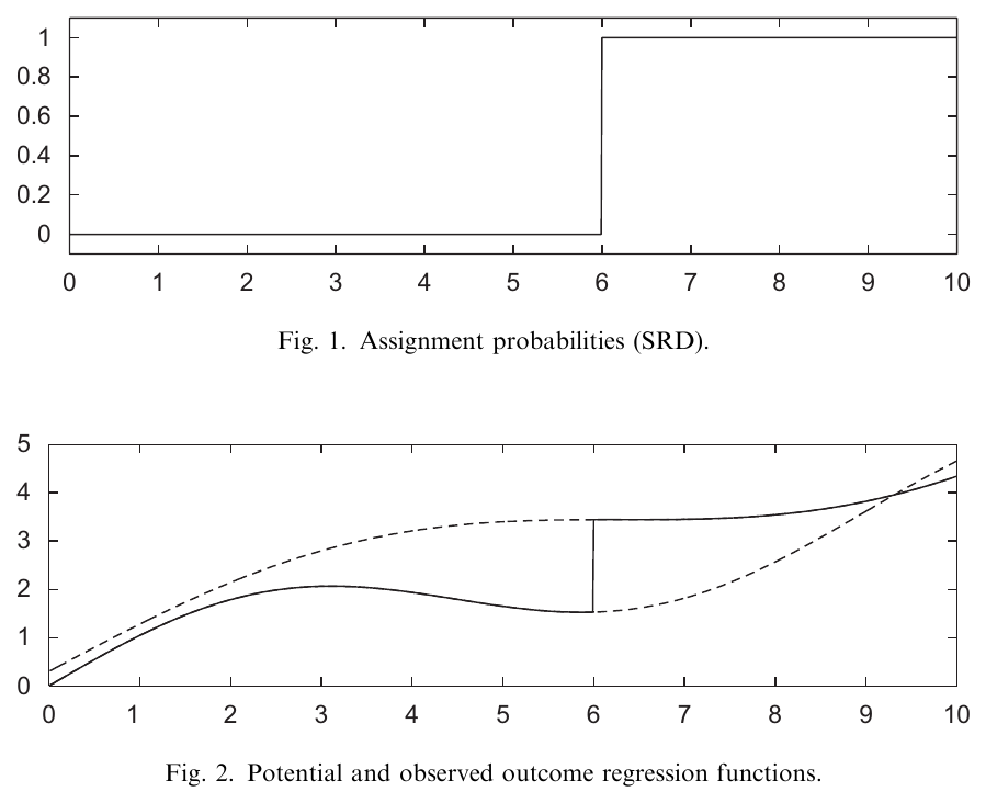
Imbens and Lemieux (2008), Figures 1–2.
The Causal Effect at the Cutoff
Using our potential-outcome notation, define
\[\rho=E\left[Y_i^1-Y_i^0\mid X_i=x_0\right].\]
The observed outcome is
\[Y_i=D_iY_i^1+\left(1-D_i\right)Y_i^0.\]
To the right of the cutoff we observe treated outcomes. To the left we observe untreated outcomes.
With a continuously distributed score, identification uses the limiting conditional means as we approach \(x_0\) from each side.
The effect is local to the cutoff. We cannot observe both potential outcomes for a person at the cutoff. Even a very large sample does not solve that missing-counterfactual problem directly. Continuity supplies the connection between the two sides. In applications with a discrete score, such as integer enrolment, there are gaps between possible values and this limiting argument requires additional care.
The Continuity Assumption
For each potential outcome, the conditional mean approaches the same value from either side of the cutoff:
\[\lim_{x\uparrow x_0}E\left[Y_i^0\mid X_i=x\right] =\lim_{x\downarrow x_0}E\left[Y_i^0\mid X_i=x\right] =E\left[Y_i^0\mid X_i=x_0\right].\]
\[\lim_{x\uparrow x_0}E\left[Y_i^1\mid X_i=x\right] =\lim_{x\downarrow x_0}E\left[Y_i^1\mid X_i=x\right] =E\left[Y_i^1\mid X_i=x_0\right].\]
Average outcomes under either treatment state would change smoothly as we cross the cutoff.
The two potential-outcome means can differ from one another. That difference at \(x_0\) is the treatment effect.
Here \(x\uparrow x_0\) means approaching the cutoff from below, and \(x\downarrow x_0\) means approaching it from above. The first equation concerns the mean outcome if everyone were untreated. The second concerns the mean outcome if everyone were treated. In each case the left and right limits equal the conditional mean at the cutoff.
Below the cutoff we observe \(Y_i^0\), and above it we observe \(Y_i^1\). Continuity lets us use the limiting mean from below as the untreated counterfactual at the cutoff for the comparison with those approaching from above. The jump in observed conditional mean outcomes therefore identifies the treatment effect at the cutoff.
Other determinants of the outcome must not generate their own discontinuity at \(x_0\). Another policy changing at the same cutoff would complicate the interpretation of the jump. In an election application, ask whether candidate or constituency characteristics change abruptly at a zero winning margin, and whether votes can be precisely manipulated around zero.
Continuity of the potential-outcome conditional means is sufficient for identifying the average effect at the cutoff. This does not require continuity of the entire conditional distributions.
Deriving the Sharp RD Effect
Immediately to the right, \(D_i=1\). By continuity,
\[\lim_{x\downarrow x_0}E\left[Y_i\mid X_i=x\right] =E\left[Y_i^1\mid X_i=x_0\right].\]
Immediately to the left, \(D_i=0\). By continuity,
\[\lim_{x\uparrow x_0}E\left[Y_i\mid X_i=x\right] =E\left[Y_i^0\mid X_i=x_0\right].\]
Subtracting gives
\[\rho=\lim_{x\downarrow x_0}E\left[Y_i\mid X_i=x\right] -\lim_{x\uparrow x_0}E\left[Y_i\mid X_i=x\right].\]
Here \(x\downarrow x_0\) means approaching the cutoff from above, while \(x\uparrow x_0\) means approaching it from below. The observed jump equals the causal effect because continuity lets us replace the two limits with the two potential-outcome means at the same cutoff.
2. Graphical evidence and close elections
Graphical Analysis: Outcomes
Divide the running variable into bins \([b_k,b_{k+1})\), with the cutoff as a bin boundary.
The number of observations in bin \(k\) is
\[N_k=\sum_{i=1}^{n}1\left(b_k\le X_i<b_{k+1}\right).\]
The mean outcome in that bin is
\[\bar Y_k=\frac{1}{N_k}\sum_{i=1}^{n}Y_i1\left(b_k\le X_i<b_{k+1}\right).\]
Plot \(\bar Y_k\) against the midpoint \(\widetilde b_k=\left(b_k+b_{k+1}\right)/2\).
No bin should cross the cutoff.
Each plotted point summarises several observations. For equally spaced bins of width \(h_b\), we can set \(b_k=x_0+(k-K_0-1)h_b\) for \(k=1,\ldots,K_0+K_1+1\). This places \(K_0\) bins below and \(K_1\) bins above the cutoff. Changing the bin width changes the amount of visual smoothing. The bin width used for the graph is distinct from the estimation bandwidth introduced below.
Lee (2008): Elections and Incumbency
Lee studies US House elections and the effect of winning office on subsequent electoral success.
- Running variable: the Democratic winning margin in the current election.
- Cutoff: a margin of zero.
- Treatment: a Democratic victory in the current election.
- Outcomes: subsequent candidacy, vote share, and victory.
Why should narrow winners and narrow losers be informative about the effect of incumbency?
Lee: Outcome Plot
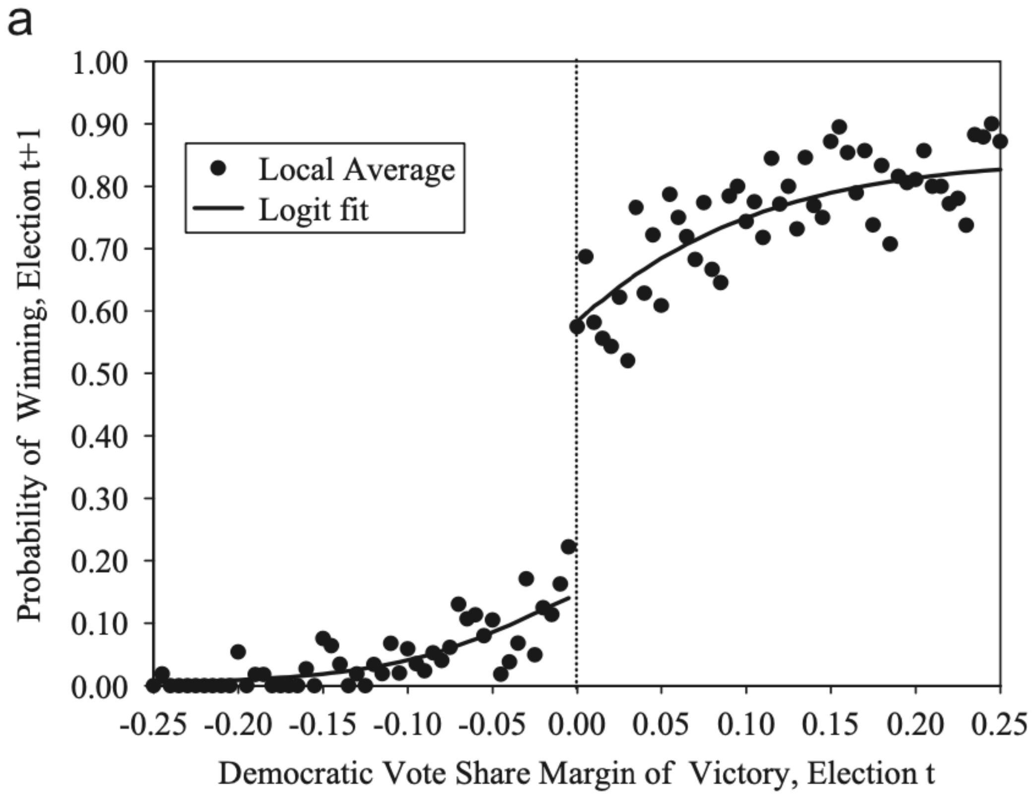
Lee (2008), outcome plot reproduced in the original slides.
Graphical Analysis: Predetermined Covariates
For a predetermined characteristic \(W_{mi}\), calculate
\[\bar W_{mk}=\frac{1}{N_k}\sum_{i=1}^{n}W_{mi}1\left(b_k\le X_i<b_{k+1}\right).\]
Plot these means against the same bin midpoints.
A discontinuity in characteristics determined before treatment raises questions about the comparability of observations on the two sides.
The institutional explanation and these diagnostic checks support the continuity assumption.
Lee: Past Electoral Victories
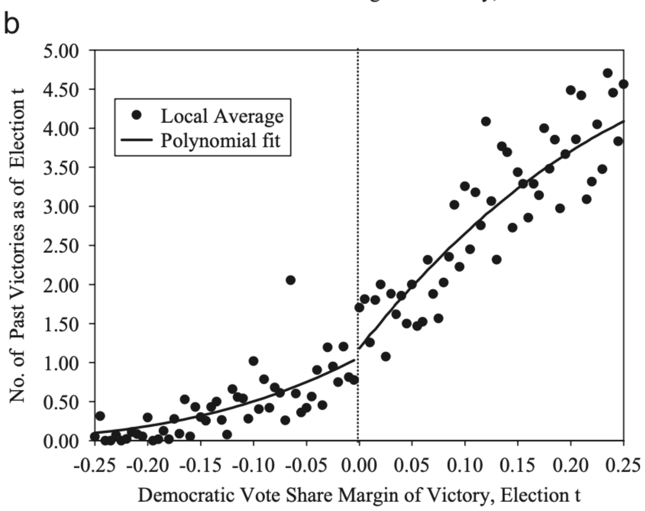
Lee (2008), predetermined electoral history.
Lee: Subsequent Candidacy
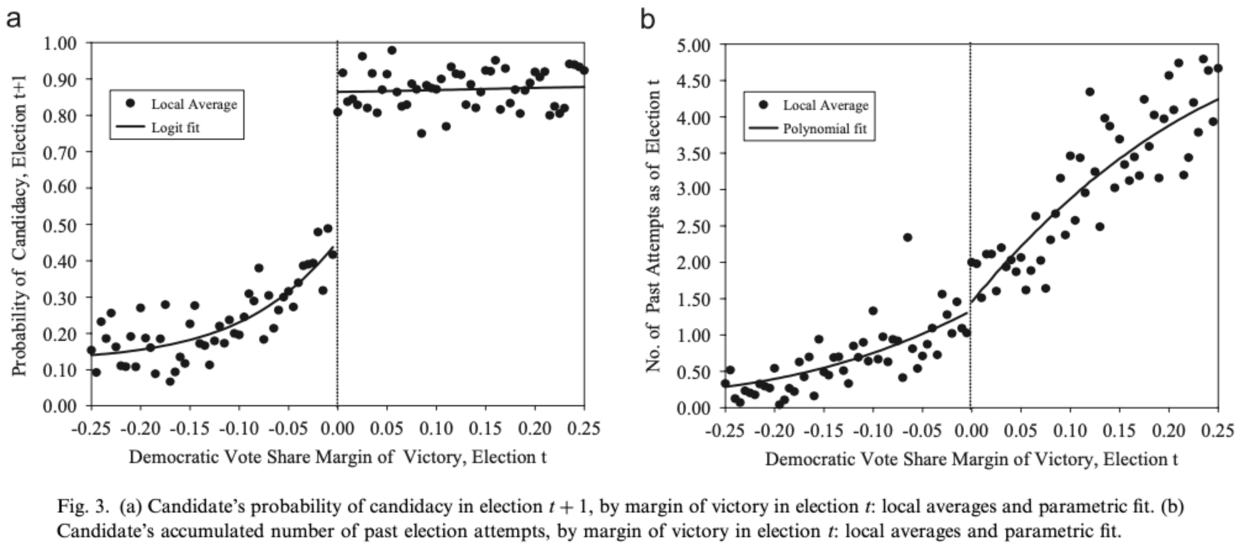
Lee (2008), Figure 3.
Lee: Subsequent Democratic Vote Share
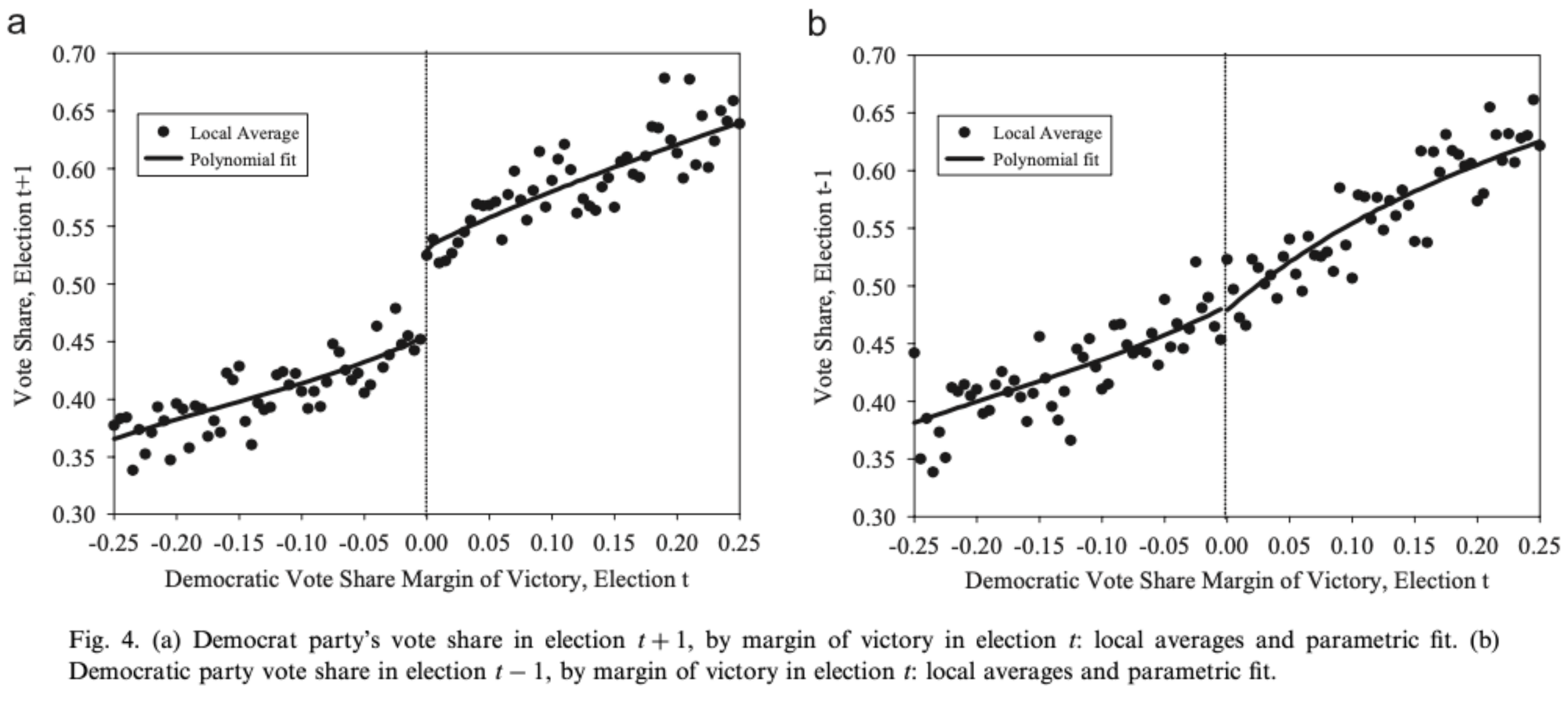
Lee (2008), Figure 4.
Lee: Subsequent Democratic Victory
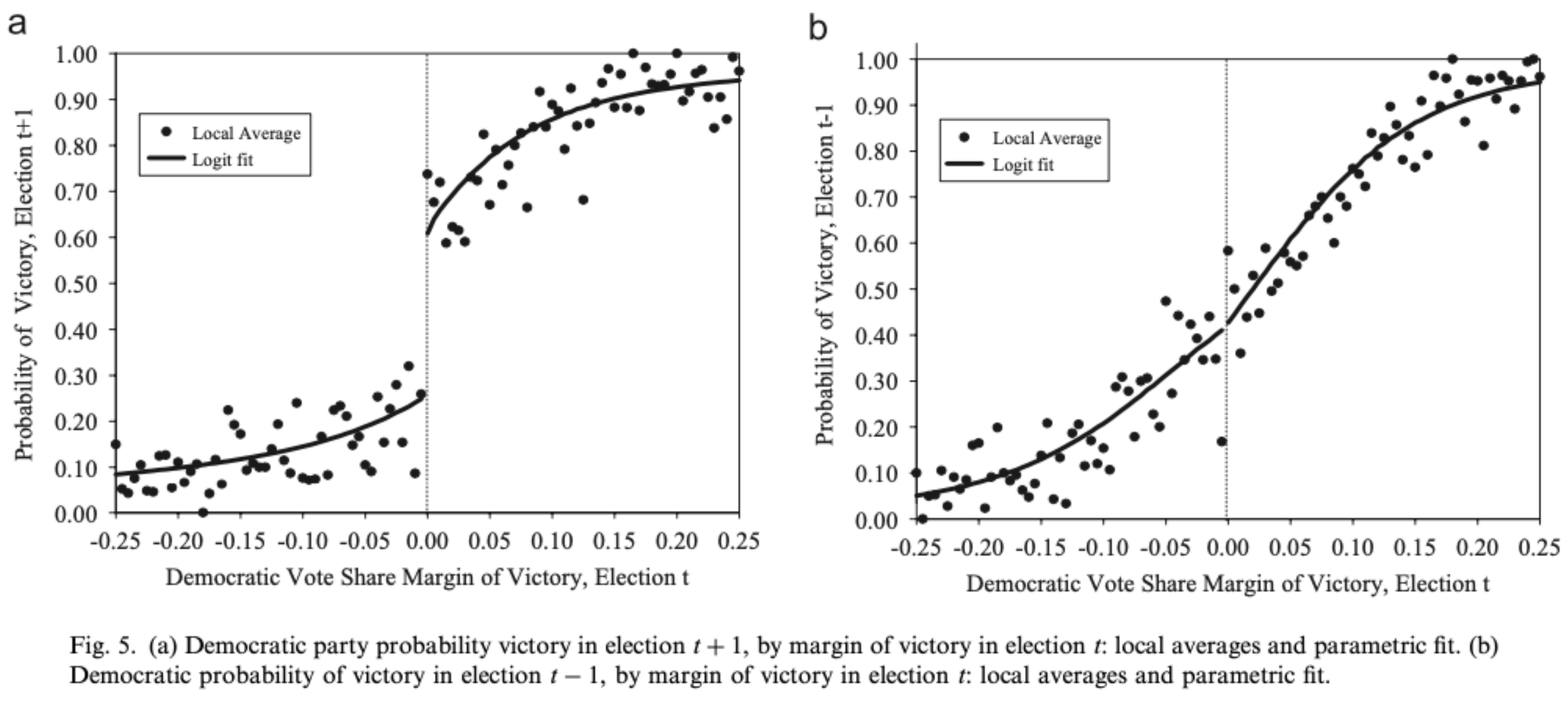
Lee (2008), Figure 5.
3. Estimating the discontinuity
RD as a Regression
Centre the running variable: \(R_i=X_i-x_0\).
Suppose, locally,
\[E\left[Y_i^0\mid X_i\right]=\beta_0+\beta_1R_i,\qquad Y_i^1=Y_i^0+\rho.\]
Then
\[Y_i=\beta_0+\beta_1R_i+\rho D_i+\epsilon_i.\]
Here \(\epsilon_i=Y_i^0-E\left[Y_i^0\mid X_i\right]\) is the disturbance: the difference between an individual’s untreated outcome and its conditional mean. Thus \(E\left[\epsilon_i\mid X_i\right]=0\).
At \(R_i=0\), the fitted untreated outcome is \(\beta_0\) and the fitted treated outcome is \(\beta_0+\rho\).
The difference between the intercepts is the treatment effect at the cutoff.
The constant-effect assumption is a convenient way to introduce this regression. Identification of the effect at the cutoff does not require treatment effects to be constant throughout the population. Centring is important: it makes the treatment coefficient the jump at the actual threshold, even when the original cutoff is far from zero.
Allowing Different Slopes
Allow the relationship between the score and the outcome to differ on the two sides:
\[Y_i=\beta_0+\rho D_i+\beta_1R_i+\gamma_1D_iR_i+\epsilon_i.\]
- Below the cutoff: intercept \(\beta_0\), slope \(\beta_1\).
- Above the cutoff: intercept \(\beta_0+\rho\), slope \(\beta_1+\gamma_1\).
Because \(R_i=0\) at the cutoff, the interaction contributes zero there. The jump remains \(\rho\).
Polynomial Regression
If the conditional mean is curved, we can allow powers of the centred score:
\[Y_i=\beta_0+\rho D_i+ \sum_{j=1}^{p}\beta_jR_i^j+ \sum_{j=1}^{p}\gamma_jD_iR_i^j+\epsilon_i.\]
The two sums allow different shapes on either side of the cutoff.
At \(R_i=0\), all the terms in those sums are zero, so \(\rho\) remains the jump.
A high-order polynomial over a wide range can fit poorly near the cutoff and confuse curvature with a discontinuity.
Local Regression
Use observations within a bandwidth \(h\):
\[-h<R_i<h.\]
Fit a separate low-order polynomial on each side and evaluate both at \(R_i=0\).
- A smaller bandwidth uses more local information, but fewer observations.
- A larger bandwidth improves precision, but fitting a simple function over a wider range can introduce more approximation bias.
The bandwidth determines which observations inform the estimated jump.
Continuity implies that conditional means in increasingly narrow windows approach the corresponding limits at the cutoff. In a finite sample we need enough observations to estimate those limits. Local linear regression also allows an underlying slope within each window rather than treating everyone in it as having the same expected outcome.
What Is a Bandwidth?
The bandwidth is the distance from the cutoff within which we use observations to estimate the jump.
Suppose treatment starts at a score of 50:
- With \(h=10\), use scores between 40 and 60.
- With \(h=5\), use scores between 45 and 55.
A smaller bandwidth brings the comparison closer to the cutoff and leaves fewer observations with which to estimate the effect.
The bandwidth is measured in the same units as the running variable. Here \(h=10\) describes ten score points on each side, so the complete window is twenty points wide. A local linear regression fits a separate line within each side of that window and compares the lines at 50. The bandwidth used for estimation and the bin width used to draw a graph serve different purposes.
What Is a Kernel?
A kernel is a rule for assigning weights according to distance from the cutoff.
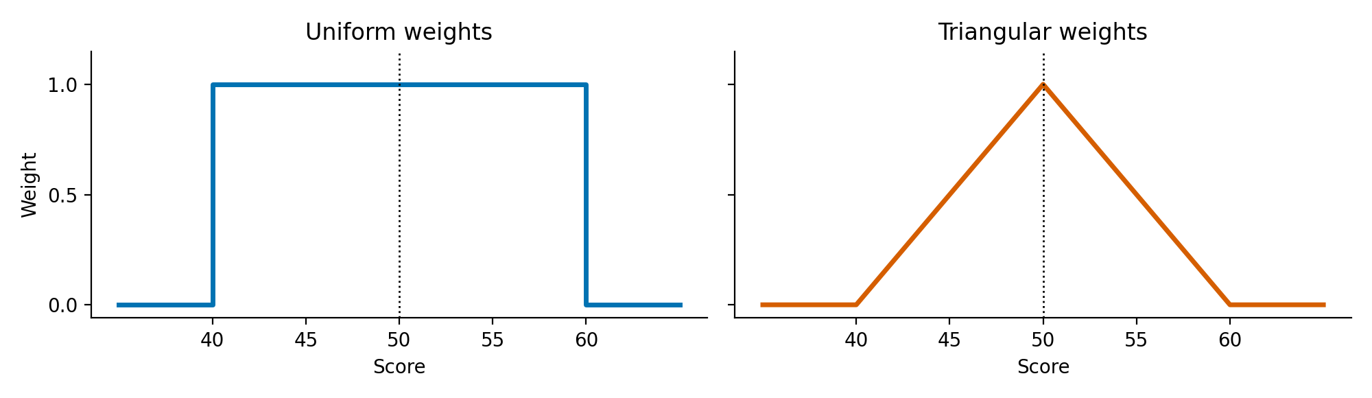
Within the same bandwidth, uniform weights are equal. Triangular weights decline as we move away from the cutoff.
With a cutoff of 50 and bandwidth of 10, triangular weights are 1 at 50, 0.5 at 45 and 55, and zero at 40 and 60. Observations outside the window receive zero weight. Uniform weights instead give every observation inside the window the same weight. Thus the bandwidth determines the window and the kernel determines how observations within it contribute to the fit. Multiplying all the weights by a common positive constant leaves the fitted regression unchanged. The next equation applies the weighted least squares idea from Week 2 to these distance-based weights.
Local Linear Regression with Weights
A triangular kernel gives more weight to observations closer to the cutoff:
\[w_i=\begin{cases}1-|R_i|/h & \text{if }|R_i|<h,\\0&\text{otherwise.}\end{cases}\]
Estimate the separate-slopes regression by minimising
\[\sum_{i=1}^{n}w_i\left(Y_i-\beta_0-\rho D_i-\beta_1R_i-\gamma_1D_iR_i\right)^2.\]
This is weighted least squares. The weights depend on distance from the cutoff.
In Week 2 the weights changed the composition of the comparison group. Here the weights emphasise observations near the threshold where the treatment effect is identified. A uniform kernel instead gives each observation inside the bandwidth the same weight. Modern practice usually starts with local linear estimation and a triangular kernel.
Bandwidth Choice and Inference
A data-driven bandwidth balances squared bias and variance: mean squared error.
At an MSE-optimal bandwidth, approximation bias can still be large enough to matter for confidence intervals.
Robust bias-corrected inference estimates that bias and accounts for the uncertainty from estimating the correction.
The rdrobust package implements bandwidth selection, local polynomial estimation, and robust bias-corrected inference.
Imbens and Kalyanaraman (2012) developed an influential bandwidth selector. Calonico, Cattaneo, and Titiunik (2014) developed robust bias-corrected inference. Heteroskedasticity-consistent standard errors address nonconstant disturbance variance. They alone do not account for local polynomial approximation bias. We therefore distinguish the familiar HC1 regression examples from the robust bias-corrected intervals reported by rdrobust. Trying half and twice a baseline bandwidth helps reveal sensitivity, while differences between the resulting estimates must also be judged against their uncertainty.
Predetermined Covariates
Predetermined covariates can improve precision when they predict the outcome and their conditional means are continuous at the cutoff.
Inspect their behaviour around the cutoff before adding them to the regression.
A jump in a baseline characteristic requires an explanation of the assignment process. Adding that characteristic as a control does not by itself establish continuity of the potential outcomes.
Report how the estimate and its uncertainty change when controls are included.
4. Sorting around the cutoff
Can People Manipulate the Running Variable?
Ask who can influence the recorded score, what they know about the cutoff, and why they would want to cross it.
If people who cross differ in other determinants of the outcome, the two sides may no longer provide comparable counterfactuals.
We will build an example where we know the original score, the manipulation, and the true treatment effect.
The simulation lets us inspect ability even though the researcher would ordinarily not observe it.
An Illustration
Generate an original score \(X_i^*\), ability \(A_i\), and noise \(u_i\), independently:
\[X_i^*\sim U\left(-2,2\right),\qquad A_i,u_i\sim N\left(0,1\right).\]
The true population relationships are
\[Y_i^0=10+0.5X_i^*+2A_i+u_i,\qquad Y_i^1=Y_i^0+2.\]
Initially, the recorded score is \(X_i=X_i^*\) and treatment is \(D_i=1\left(X_i\ge0\right)\).
The true treatment effect is 2.
Before Manipulation
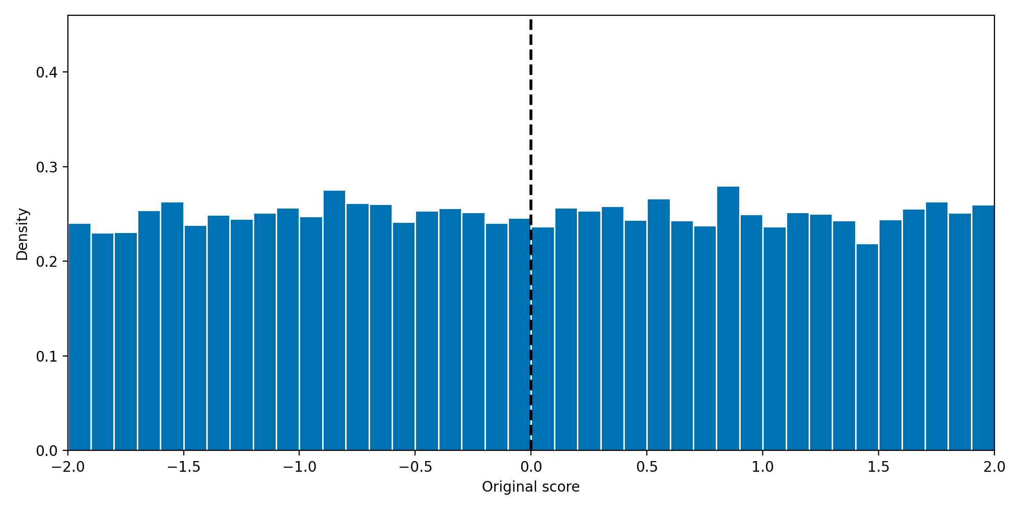
Simulated data. The dashed line is the treatment cutoff.
Who Changes Their Score?
Suppose people with \(-0.4\le X_i^*<0\) and \(A_i>0\) can change their recorded score.
For these people, set \(X_i=-X_i^*\). Everybody else retains \(X_i=X_i^*\).
For example, a person with an original score of \(-0.1\) is now recorded at \(+0.1\).
Their ability and untreated potential outcome remain unchanged. They now receive treatment, adding 2 to their outcome.
We compare this population with the same people before manipulation.
After Manipulation
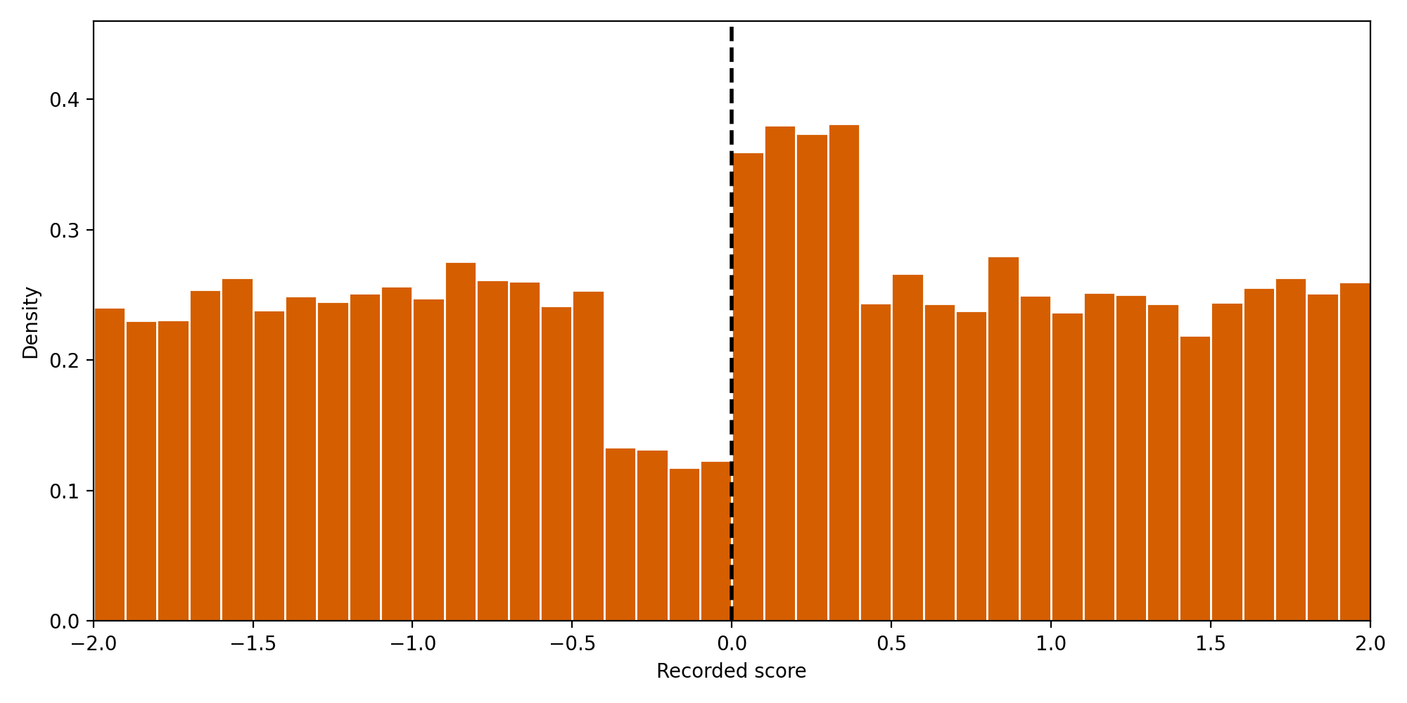
Same population, bins, and vertical scale. Only the recorded scores and resulting treatment change.
The Composition of the Groups Changes
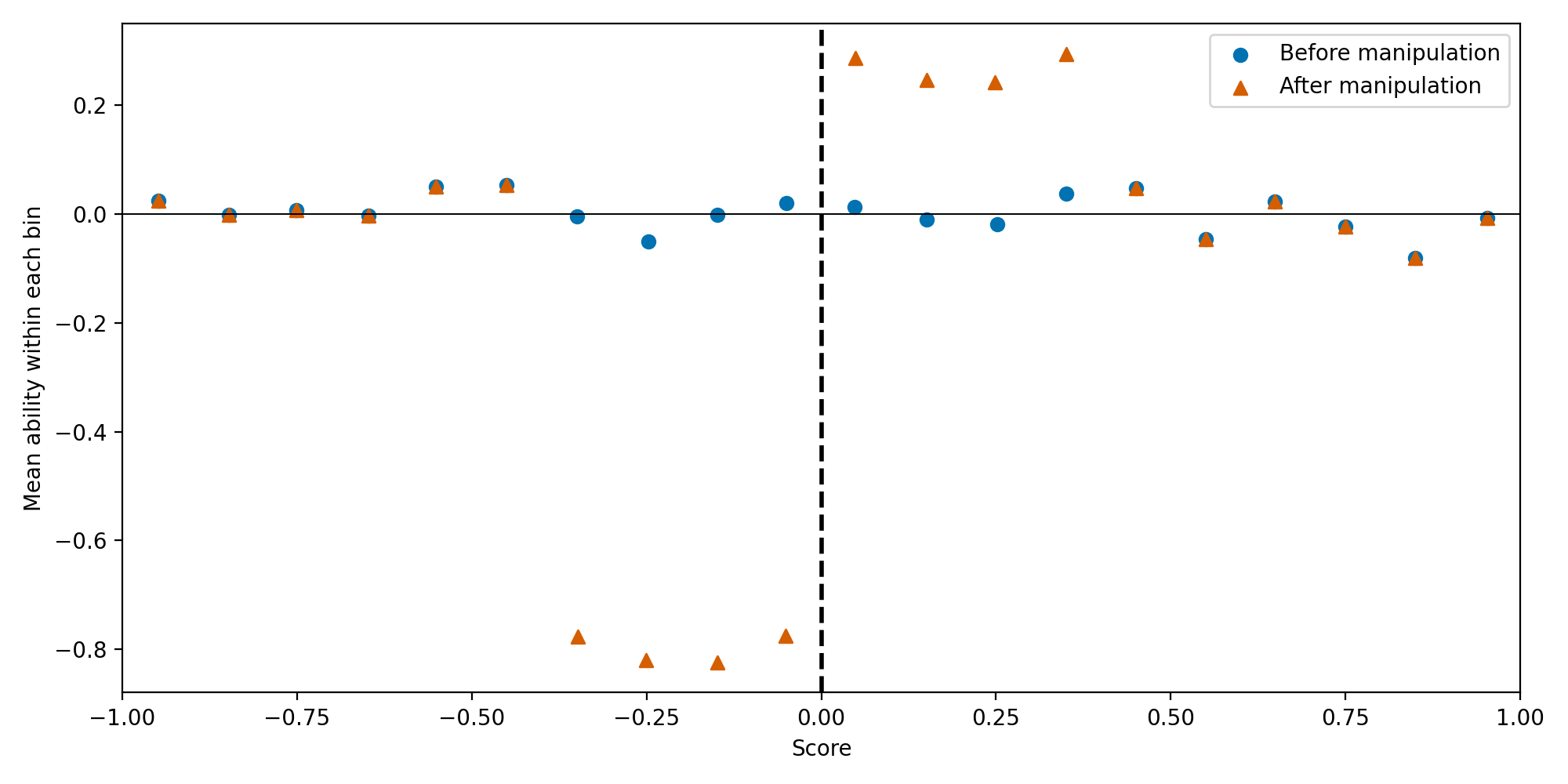
Circles: before manipulation. Triangles: after manipulation. Each point is a bin mean.
Below zero, the people with positive ability have left. Above zero, they join the original population. This produces a discontinuity in average ability. In a real application ability may be unobserved, which is why the assignment process and indirect diagnostics matter.
The Outcome Jump Changes Too
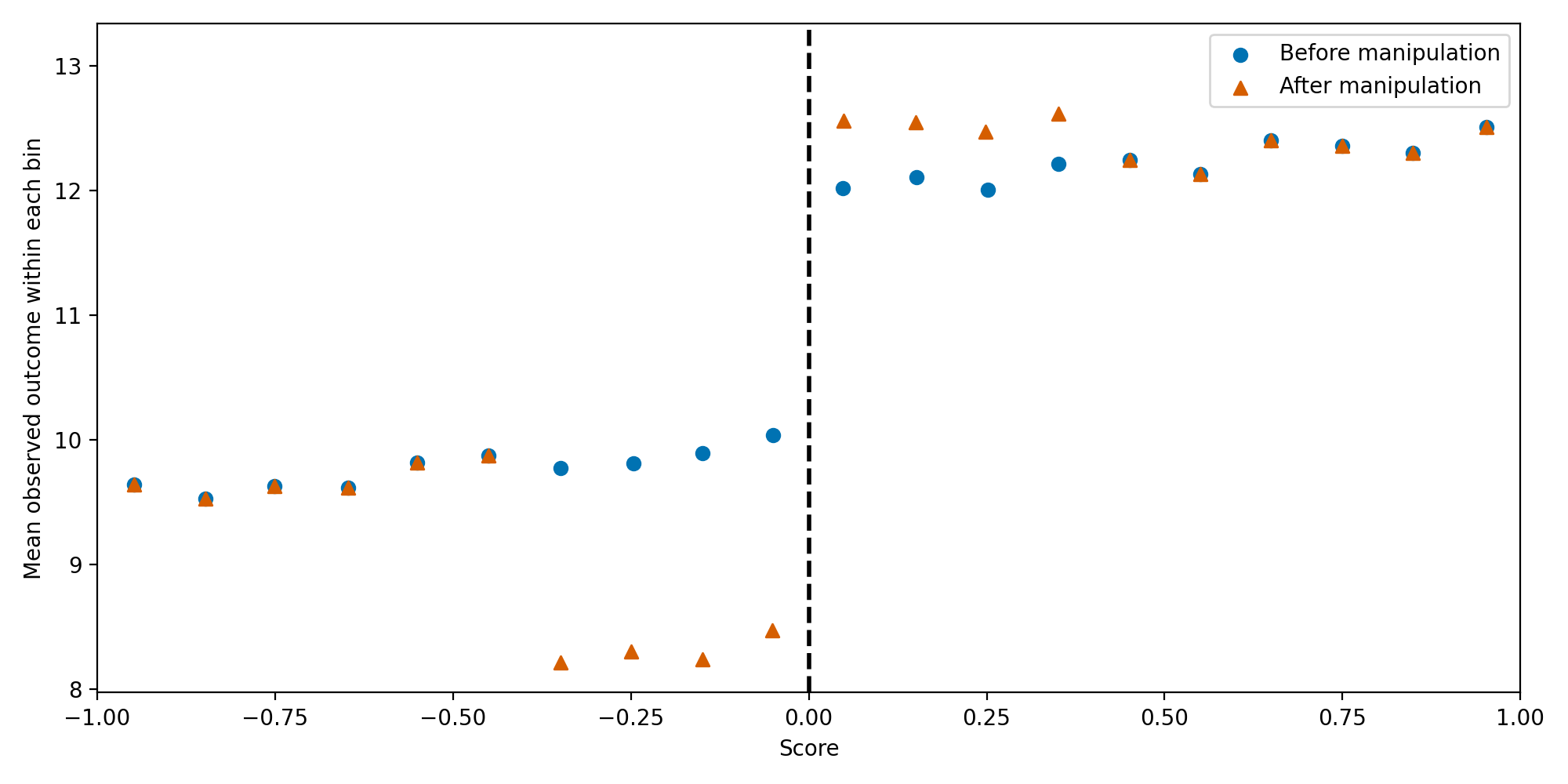
The true treatment effect remains 2 for every person.
The larger observed jump combines the treatment effect with the change in composition. The untreated conditional mean is now discontinuous at the recorded-score cutoff. An RD estimator can estimate this observed jump very precisely while failing to recover the causal effect.
What Does the Density Test Ask?
Let \(f_X\left(x\right)\) denote the density of the recorded running variable.
The null hypothesis is
\[H_0:\quad\lim_{x\uparrow x_0} f_X\left(x\right) =\lim_{x\downarrow x_0}f_X\left(x\right).\]
A histogram illustrates how observations are distributed. The test estimates the density on each side and assesses the uncertainty in the estimated difference.
The question concerns the number of observations near the cutoff, rather than their average outcome.
A density is probability per unit of the running variable. Histogram height equals the share of observations in a bin divided by its width. McCrary (2008) developed a widely used test based on the difference in estimated log densities at the cutoff. Cattaneo, Jansson, and Ma (2020) estimate density using local polynomials without preliminary binning. Their procedure still requires bandwidth selection. We use their implementation in rddensity for the Python example.
How the Cattaneo–Jansson–Ma Test Works
- Construct the empirical cumulative distribution: the proportion of observations with a score at or below each value.
- Fit local polynomials to this distribution on each side of the cutoff, using nearby observations.
- The slope of each fitted curve at the cutoff estimates the density on that side.
- Test whether the difference between the two estimated densities is zero, allowing for sampling uncertainty and smoothing bias.
The test uses individual observations, with a selected bandwidth and kernel weights. Histogram bins are used only for our descriptive graph.
The cumulative distribution is \(F_X\left(x\right)=\Pr\left(X_i\le x\right)\). Its empirical counterpart is
\[\widehat F_X\left(x\right)=\frac{1}{n}\sum_{i=1}^{n}1\left(X_i\le x\right).\]
For example, if 40 of 100 scores are at or below 48, the empirical cumulative distribution at 48 is 0.40. As we move through a range containing many observations, this cumulative proportion rises rapidly. Its slope measures how densely observations are concentrated there. For a continuous running variable, the population density is the derivative of the cumulative distribution, \(f_X\left(x\right)=F_X'\left(x\right)\).
The empirical distribution is a staircase. Cattaneo, Jansson, and Ma smooth it locally using polynomial regressions. The slopes of the fitted curves at the cutoff provide left- and right-hand density estimates. A density discontinuity appears as a change in slope of the cumulative distribution. The cumulative distribution itself can remain continuous.
The null hypothesis is equality of the two limiting densities. Conceptually, the statistic is the estimated difference divided by its estimated standard error:
\[T=\frac{\widehat f_{+}\left(x_0\right)-\widehat f_{-}\left(x_0\right)}{\widehat{\operatorname{se}}\left[\widehat f_{+}\left(x_0\right)-\widehat f_{-}\left(x_0\right)\right]}.\]
Here \(+\) denotes the estimate from above the cutoff and \(-\) the estimate from below. The implementation uses higher-order fitting to account for smoothing bias and a standard error appropriate to density estimation. The default Python output used below reports a two-sided test with jackknife standard errors. The package selects bandwidths and uses triangular weights by default. No histogram bins enter the calculation. See the rddensity documentation for details.
A small p-value indicates evidence against equal densities at the cutoff. Investigate whether sorting, manipulation, or the way the score is recorded could explain the difference. A larger p-value means that the test has not detected a discontinuity. Its ability to detect a substantively important difference depends on precision. Consider this evidence alongside the institutional setting and checks on predetermined characteristics.
Density-Test Results
| Recorded score | Test statistic | \(p\)-value |
|---|---|---|
| Before manipulation | −0.697 | 0.486 |
| After manipulation | 6.205 | \(<0.001\) |
The sample contains 20,000 people. The test uses the Cattaneo–Jansson–Ma procedure and its default bandwidth selection.
We detect a density discontinuity after manipulation. The simulation shows why that discontinuity accompanies a change in the composition of the groups.
Interpreting the Density Test
- Reject continuity: investigate sorting, the recording process, and the institutional rules.
- Do not reject: the data provide no statistically detectable density jump at the cutoff.
A smooth density does not establish continuity of unobserved determinants of the outcome. Some forms of sorting can leave the density smooth.
Rounding and discrete scores also affect how we interpret the graph and choose a test.
Combine the diagnostic with the institutional explanation and predetermined-covariate checks.
NoteYour turn
In the simulation, explain why the outcome jump changes even though the treatment effect stays at 2. What can a researcher learn from the score distribution when ability is unobserved? What further evidence would you seek?
5. Islamic rule and education in Turkey
NoteYour turn
Explain the research question, the unit of observation, the timing of treatment and outcomes, and how the election and census data are combined.
Meyersson (2014): Question and Data
Does electing an Islamic mayor affect educational attainment?
The study links the 1994 municipal elections in Turkey to the 2000 Population Census.
- Treatment is an Islamic mayor winning the 1994 election.
- A main outcome is the share of women aged 15–20 in 2000 who completed high school.
- The municipality is the unit of analysis.
Comparing all municipalities with Islamic and secular mayors could reflect substantial differences in their populations.
NoteYour turn
Define the running variable, cutoff, treatment and local comparison. Why is a 50 percent vote-share cutoff inappropriate in these multiparty elections? State the continuity assumption in the context of educational attainment.
Meyersson: The Assignment Rule
Define the Islamic winning margin as
\[X_i=\text{largest Islamic party vote share}_i -\text{largest secular party vote share}_i.\]
A positive margin means an Islamic party wins. The cutoff is zero.
Compare municipalities where an Islamic party narrowly won with those where it narrowly lost.
The design requires that expected potential educational outcomes vary continuously with this margin at zero.
NoteYour turn
Use Figure 3 and the pre-treatment panels of Figure 4 to assess comparability near the cutoff. Check when each characteristic was measured. Which evidence predates the election, and which could itself be affected by treatment?
Meyersson: Figure 3
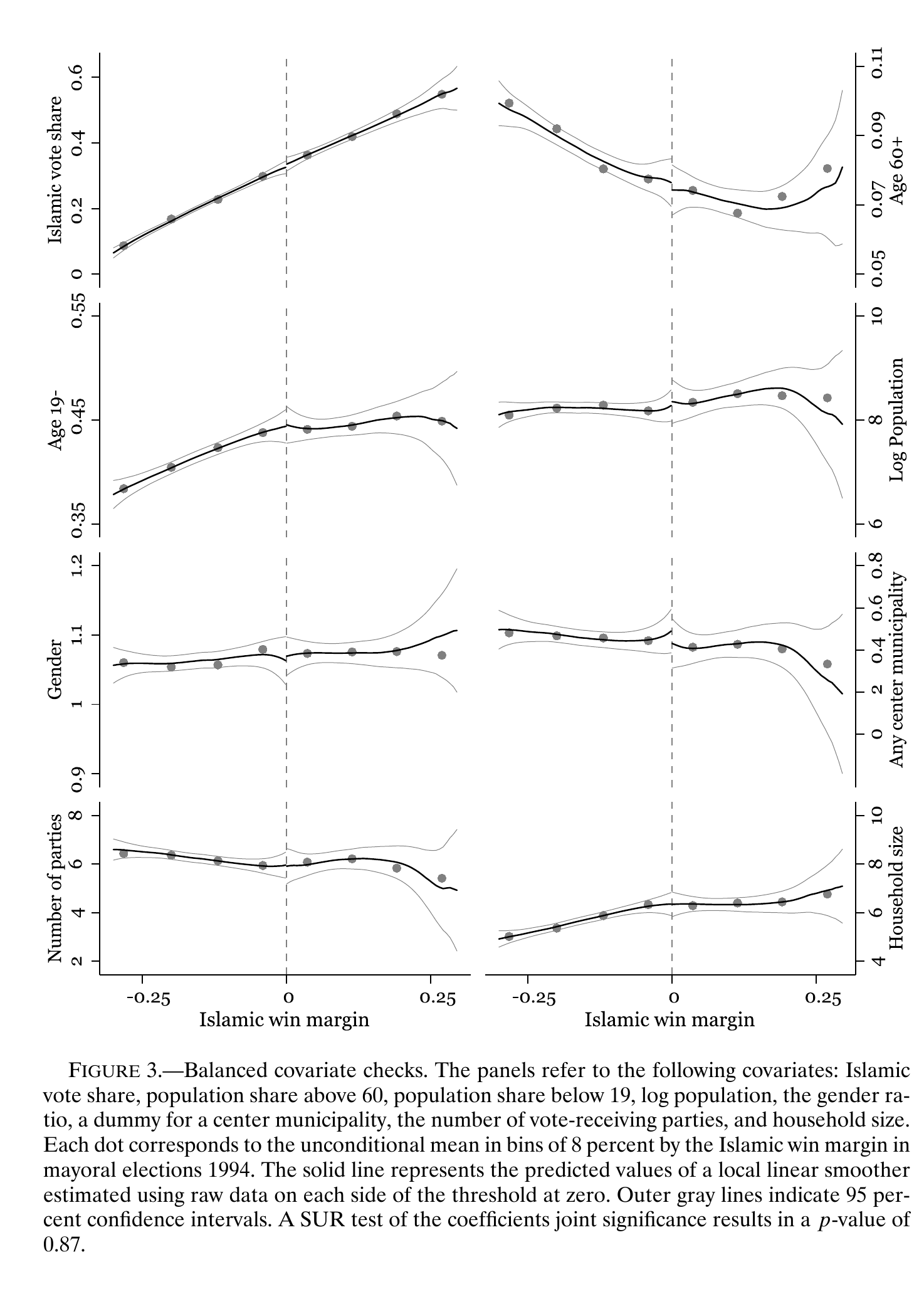
Meyersson (2014), Figure 3. Covariate checks.
Some characteristics come from the 2000 census, after the election. Their timing matters when interpreting balance. The 1990 educational outcomes in Figure 4 provide a check that clearly predates treatment.
NoteYour turn
Explain the outcomes and dates in the four panels. Which panels concern the effect of treatment and which provide a check on the design? Interpret the size and direction of the discontinuities.
Meyersson: Figure 4
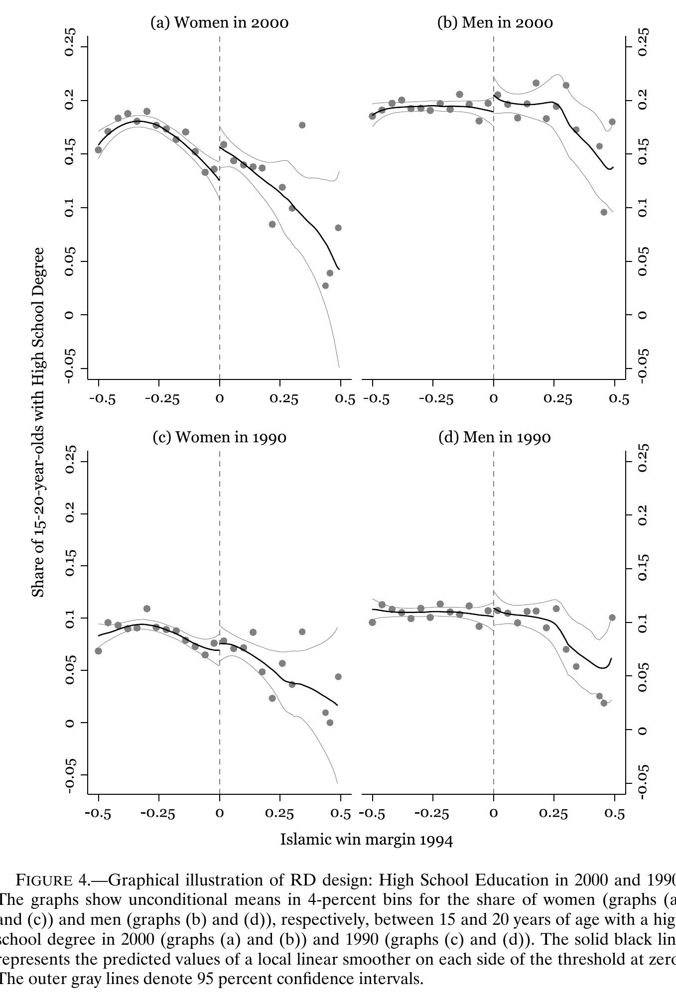
Meyersson (2014), Figure 4. High school education in 2000 and 1990.
NoteYour turn
Compare the full-sample estimates with the RD estimates in columns 3–4. Interpret the units, uncertainty and bandwidth sensitivity. Compare women and men using Panels A–C.
Meyersson: Table II, Panel A
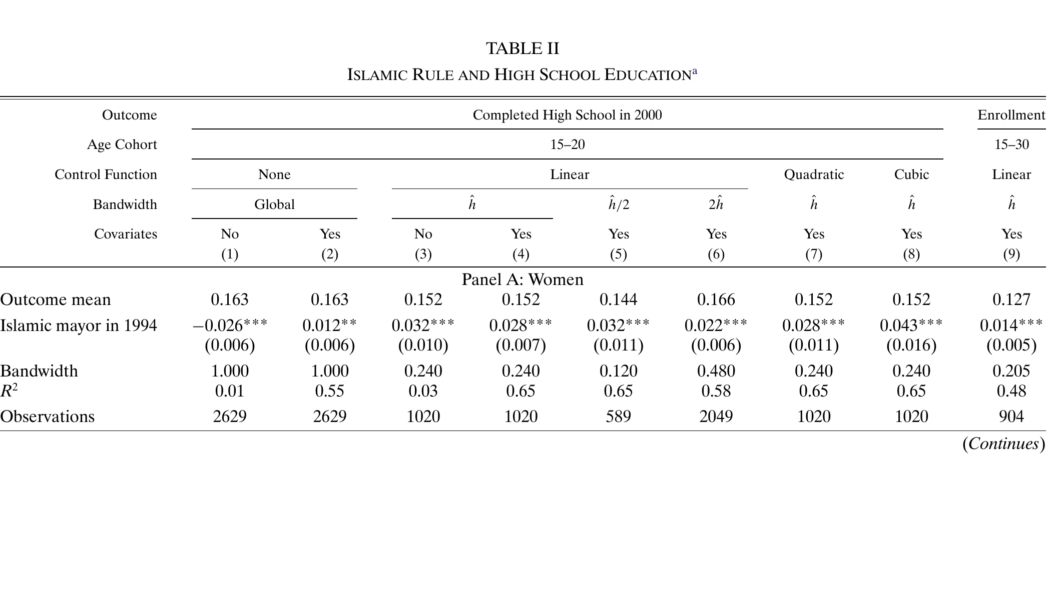
Meyersson (2014), Table II. Women.
Meyersson: Table II, Panels B–C
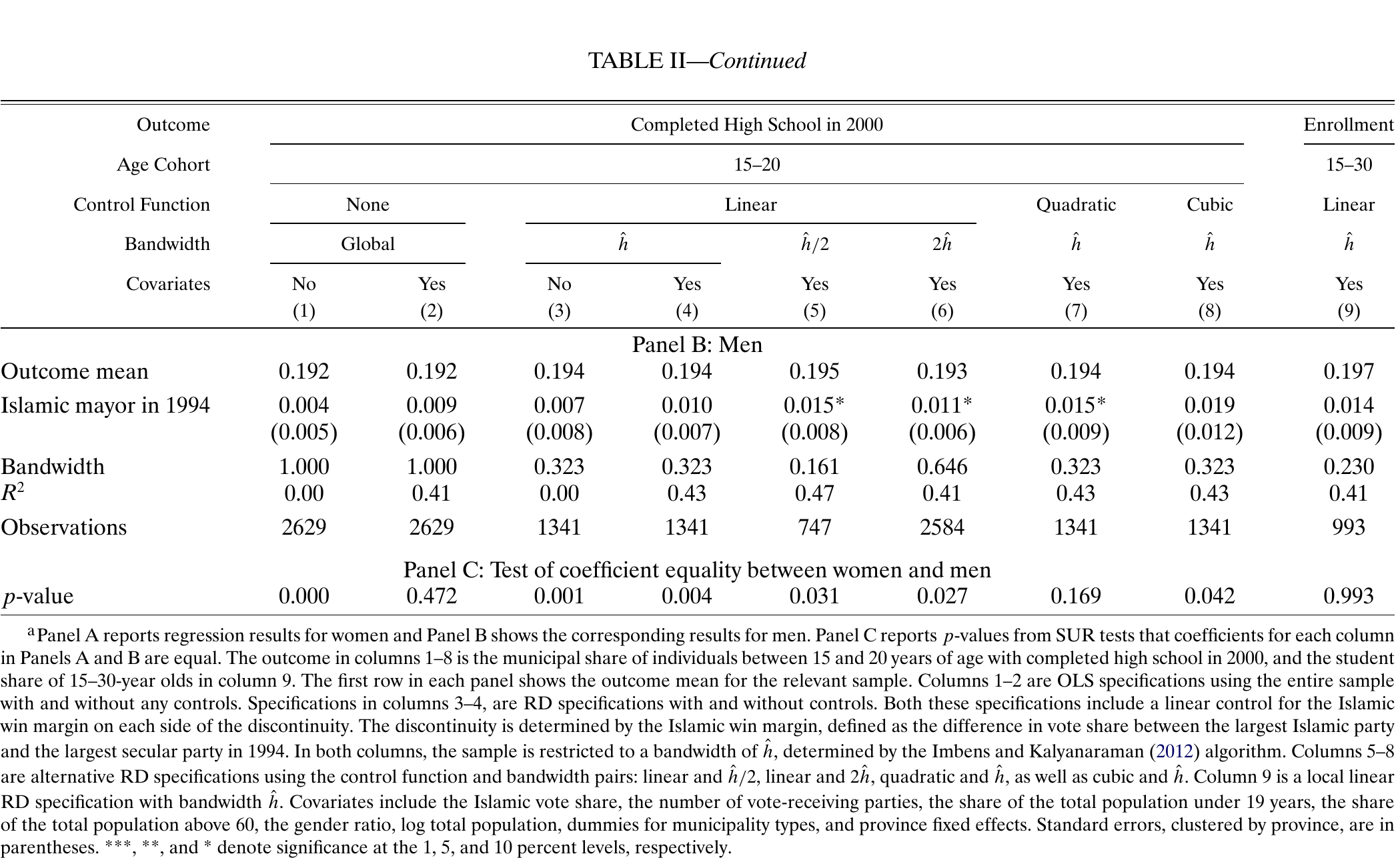
Meyersson (2014), Table II, continued. Men and tests of differences.
Interpreting the Policy Effect
The comparison identifies the effect of electing an Islamic mayor in municipalities near the electoral threshold.
That treatment changes a bundle of policies, practices and political representation.
For discussion: How far can the results distinguish the mechanisms through which education changes? To which other municipalities, elections or policy reforms would you apply the findings?
Table II reports province-clustered standard errors. In Panel A, column 3 estimates a 0.032 increase in the completion share, or 3.2 percentage points, with a standard error of 0.010. Column 4 adds covariates and estimates 0.028 with a standard error of 0.007. The paper discusses barriers to educational participation, including restrictions on religious expression. Distinguishing these mechanisms requires evidence beyond the electoral discontinuity itself.
6. Fuzzy RD and instrumental variables
Fuzzy Regression Discontinuity
Sometimes crossing the cutoff changes the probability of treatment without determining treatment completely.
\[\lim_{x\downarrow x_0}E\left[D_i\mid X_i=x\right] \ne\lim_{x\uparrow x_0}E\left[D_i\mid X_i=x\right].\]
For binary treatment, these conditional means are treatment probabilities. The jump can be smaller than 1.
The cutoff creates an instrument for treatment.
Fuzzy Discontinuity
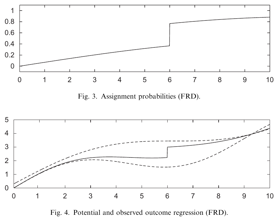
Imbens and Lemieux (2008), Figures 3–4.
The Fuzzy RD Estimand
Divide the outcome discontinuity by the treatment discontinuity:
\[\rho_{FRD}=\frac{ \lim_{x\downarrow x_0}E\left[Y_i\mid X_i=x\right]-\lim_{x\uparrow x_0}E\left[Y_i\mid X_i=x\right] }{ \lim_{x\downarrow x_0}E\left[D_i\mid X_i=x\right]-\lim_{x\uparrow x_0}E\left[D_i\mid X_i=x\right] }.\]
This is a local Wald ratio:
\[\frac{\text{reduced-form jump}}{\text{first-stage jump}}.\]
The denominator must be nonzero and estimated with sufficient precision.
What Makes the Fuzzy RD Ratio Causal?
For a binary treatment, the interpretation is a LATE at the cutoff for people whose treatment changes when eligibility changes.
We need:
- Continuity of potential outcomes and treatment behaviour through the cutoff, apart from the eligibility change.
- A nonzero first-stage discontinuity.
- Exclusion: eligibility affects the outcome through treatment.
- Monotonicity: eligibility changes treatment in the same direction for everyone at the cutoff.
Retain the well-defined-treatment and no-interference assumptions.
Let \(Z_i=1\left(X_i\ge x_0\right)\) and let \(D_i^1,D_i^0\) denote treatment under eligibility and ineligibility. With monotonicity \(D_i^1\ge D_i^0\), the denominator equals the limiting share of compliers at the cutoff. The reduced-form jump equals that share multiplied by their mean treatment effect. Dividing cancels the complier share, exactly as in the Week 3 LATE argument. Here continuity connects the limiting populations on either side, since \(Z_i\) is a deterministic function of the score.
Fuzzy RD as Two-Stage Least Squares
We estimate fuzzy RD by instrumenting actual treatment \(D_i\) with the cutoff indicator
\[Z_i=1\left(X_i\ge x_0\right).\]
This instrument is a deterministic function of the running variable: knowing \(X_i\) tells us whether \(Z_i\) is zero or one. Crossing the cutoff changes eligibility and therefore the probability of receiving treatment. Actual treatment \(D_i\) can differ from eligibility \(Z_i\).
The identifying argument comes from continuity at the cutoff. Smooth changes in the running variable are accounted for by the local regression, while the discontinuous change in eligibility supplies the instrument for treatment.
Choose a bandwidth and use observations near the cutoff. Set \(R_i=X_i-x_0\), so that \(Z_i=1\left(R_i\ge0\right)\). The local linear first stage is
\[D_i=\pi_0+\pi_1Z_i+\pi_2R_i+\pi_3Z_iR_i+v_i.\]
The outcome equation is
\[Y_i=\beta_0+\rho D_i+\beta_1R_i+\gamma_1Z_iR_i+\epsilon_i.\]
Use \(Z_i\) as the excluded instrument for \(D_i\).
Include \(R_i\) and \(Z_iR_i\) as controls in both equations. They allow separate slopes on the two sides.
Estimate the first stage and obtain
\[\widehat D_i=\widehat\pi_0+\widehat\pi_1Z_i+\widehat\pi_2R_i+\widehat\pi_3Z_iR_i.\]
The estimated second-stage regression is
\[Y_i=\widehat\beta_0+\widehat\rho\widehat D_i+\widehat\beta_1R_i+\widehat\gamma_1Z_iR_i+\widehat r_i.\]
The coefficient on predicted treatment, \(\widehat\rho\), is the fuzzy RD estimate. Here \(\widehat r_i\) is the second-stage regression residual. Use an IV routine for estimation and standard errors, as in Week 3. Both stages use the same local sample, controls and any kernel weights.
The instrument set includes the exogenous controls as well as the excluded cutoff indicator. Treating the score interactions as additional excluded instruments would impose further restrictions on their relationship with the outcome. With one endogenous treatment and one excluded cutoff indicator, the model is exactly identified. Using the same observations, weights and controls, its IV coefficient equals the ratio of the estimated reduced-form and first-stage jumps.
The Local Comparison
Restrict attention to observations near the cutoff and examine sensitivity to bandwidth.
Report the first-stage jump alongside the outcome jump and IV estimate.
A weak discontinuity in treatment creates the same denominator problem that we studied in Week 5.
With a continuous treatment such as class size, the IV coefficient describes an outcome change per unit of treatment. A binary-treatment complier interpretation requires adaptation.
Under suitable monotonicity and exclusion assumptions, an instrument for a continuous treatment identifies a weighted average of causal responses over the treatment changes induced by the instrument. A reduction of five pupils and a reduction of ten pupils need not have the same effect per pupil. We should therefore be explicit about the units of the treatment and the variation that the rule generates.
7. Class size and Maimonides’ rule
NoteYour turn
Explain the policy question, the data, and why an OLS relationship between class size and achievement may fail to identify the causal effect.
Angrist and Lavy (1999): Maimonides’ Rule
The rule limits classes to 40 pupils. As grade enrolment crosses a multiple of 40, the implied number of classes increases.
For enrolment \(e\), predicted class size is
\[m\left(e\right)=\frac{e}{\lfloor\left(e-1\right)/40\rfloor+1}.\]
For example, 40 pupils imply one class of 40. With 41 pupils, the rule implies two classes averaging 20.5.
Actual class size does not follow the rule perfectly, creating a fuzzy design.
NoteYour turn
Explain relevance, exclusion and the local comparability assumption for this rule. What changes when enrolment rises from 40 to 41? Could other school inputs change at the same point?
Actual and Predicted Class Size
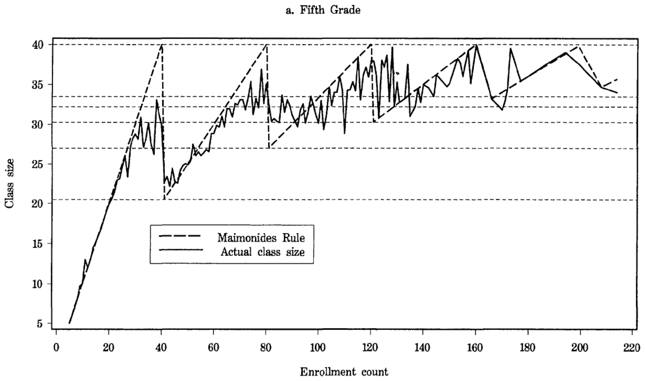
Angrist and Lavy (1999), class-size figure from the original slides.
The Reduced Form
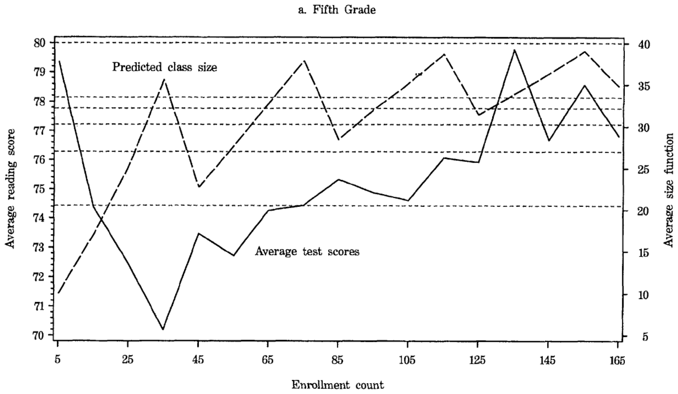
Angrist and Lavy (1999), achievement and enrolment figure from the original slides.
Estimating Equations
Let \(C_{is}\) denote class size and \(e_s\) grade enrolment. A simplified outcome equation is
\[Y_{is}=\beta_0+\rho C_{is}+f\left(e_s\right)+\sum_{j=1}^{J}\delta_jW_{jis}+\epsilon_{is}.\]
The first stage uses class size predicted by the rule:
\[C_{is}=\pi_0+\pi_1m\left(e_s\right)+g\left(e_s\right)+\sum_{j=1}^{J}\lambda_jW_{jis}+v_{is}.\]
The controls allow enrolment and background characteristics to be related to achievement. The discontinuities in the rule provide the excluded variation.
The original paper uses several enrolment specifications and discontinuity samples. Read the exact controls and sample definitions in each table. Around a single threshold, we can instead use the local cutoff-indicator specification developed above. Because larger enrolment just above a threshold can induce smaller classes, the first-stage direction must be interpreted carefully.
The Original Outcome Equation
Using the notation in Angrist and Lavy, but writing the controls as a sum,
\[Y_{isc}=\sum_{j=1}^{J}\beta_jX_{js}+\alpha n_{sc}+\mu_s+\epsilon_{isc}.\]
Here \(i\) indexes pupils, \(s\) schools and \(c\) classes. \(n_{sc}\) is class size and \(X_{js}\) contains the observed school controls, including an intercept.
The unobserved school component \(\mu_s\) can be related to class size. This is one reason that the OLS coefficient on class size may be biased.
The Original First Stage
In the paper’s notation, the first stage is
\[n_{sc}=\sum_{j=1}^{J}\pi_{0j}X_{js}+\pi_1 f_{sc}+\xi_{sc}.\]
The excluded instrument \(f_{sc}\) is predicted class size from Maimonides’ rule:
\[f_{sc}=\frac{e_s}{\lfloor\left(e_s-1\right)/40\rfloor+1}.\]
The included exogenous controls appear in both equations. The first stage isolates the class-size variation predicted by the rule, conditional on those controls.
NoteYour turn
Compare OLS and IV estimates, their units and uncertainty. Identify the instruments, enrolment controls and discontinuity samples. Explain what variation identifies the IV effect.
Angrist and Lavy: Table II
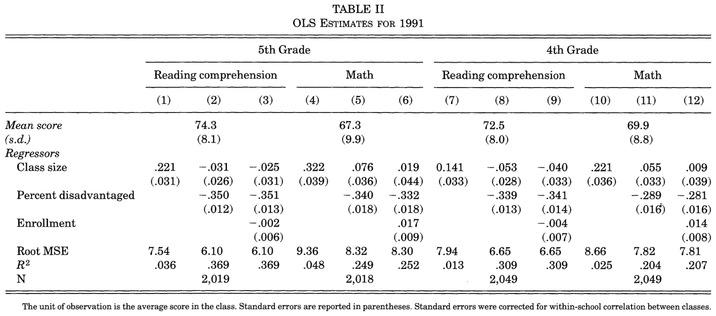
Angrist and Lavy (1999), Table II. OLS results.
Angrist and Lavy: Table IV
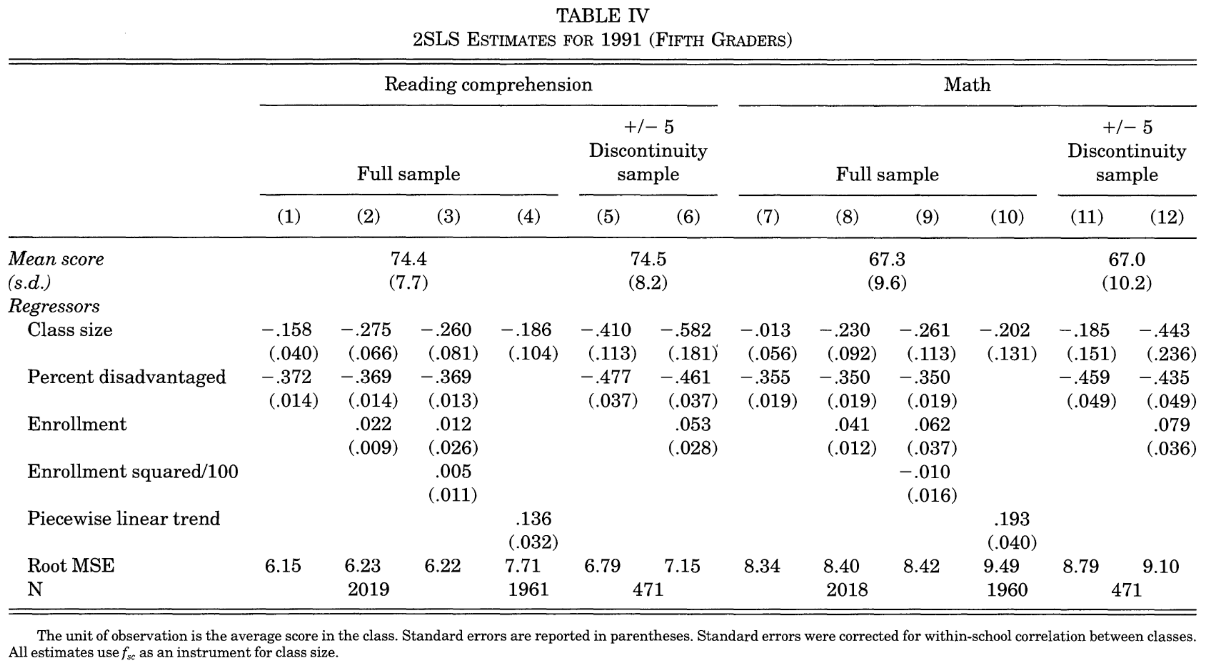
Angrist and Lavy (1999), Table IV. IV results.
8. Revisiting the design
NoteYour turn
What do the newer data allow the authors to investigate? Explain why the later study can inform our interpretation of the earlier findings even when the policy rule is unchanged.
Maimonides’ Rule Redux (2019)
Angrist, Lavy, Leder-Luis and Shany revisit the design with much larger Israeli samples from 2002–2011.
The rule continues to predict class size, while the newer achievement estimates are close to zero.
The data also reveal manipulation of reported enrolment near the thresholds.
The authors construct an alternative enrolment measure using birthdays and examine whether the findings change.
Compare the estimates and their confidence intervals with the original results rather than treating a nonsignificant coefficient as proof of an exactly zero effect. The follow-up also changes what we know about the assignment process. The birthday-based instrument gives an alternative source of predicted class size that does not use the same reported enrolment measure.
NoteYour turn
Explain the enrolment distribution around the thresholds. Who might influence reported enrolment, and what incentive would they have? Connect the figure to our simulation.
Redux: Figure 1
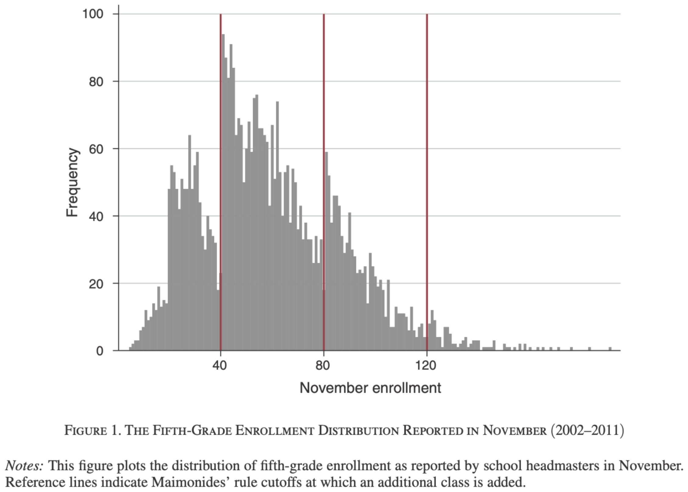
Angrist, Lavy, Leder-Luis and Shany (2019), Figure 1.
NoteYour turn
Explain how birthday-based imputed enrolment changes the construction of the instrument. What assumptions does this approach require?
Redux: Figure 2
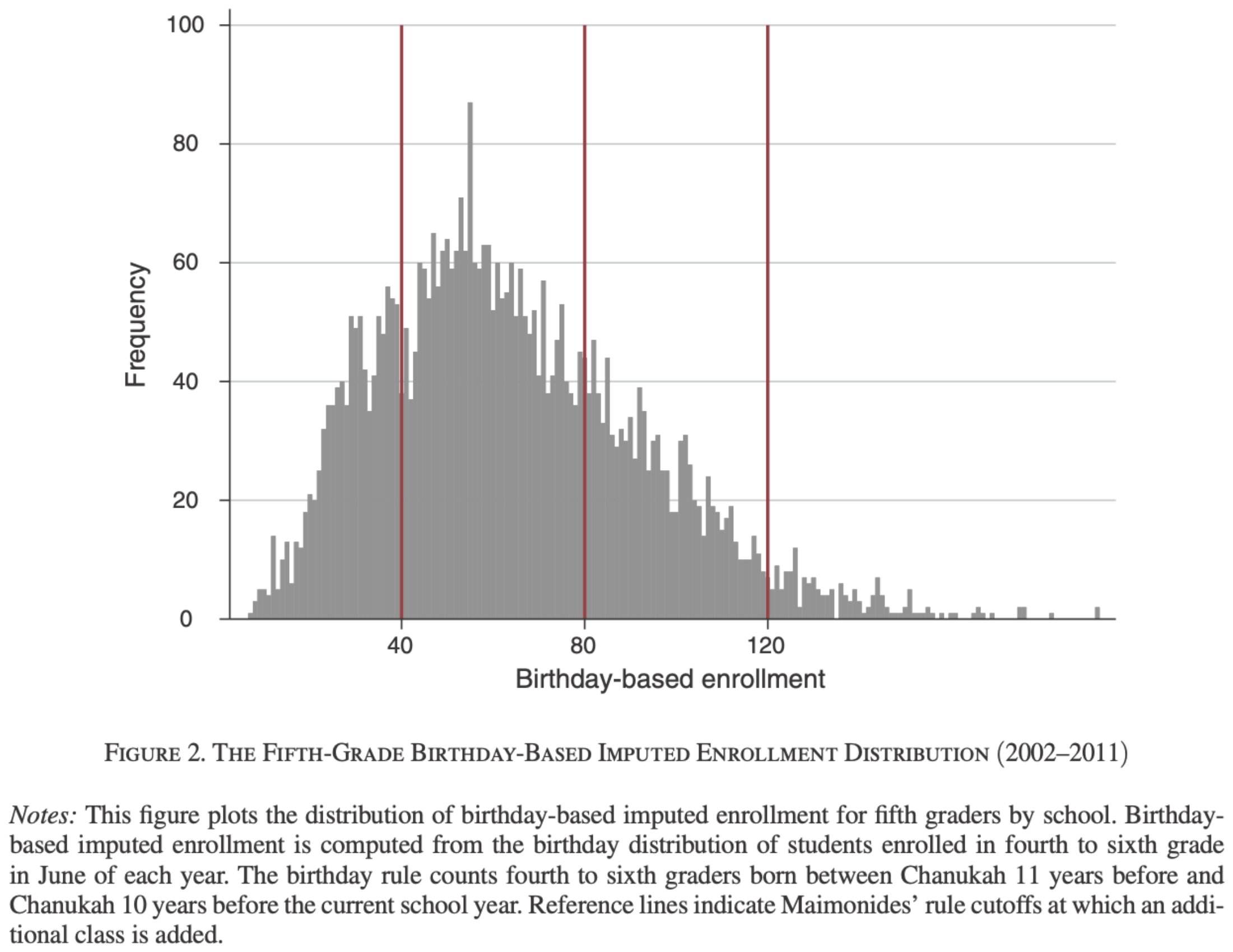
Angrist, Lavy, Leder-Luis and Shany (2019), Figure 2.
NoteYour turn
Compare the November-enrolment and birthday-based results. Discuss the first-stage evidence, the estimated effects and uncertainty, and what the comparison teaches us about the original design.
Redux: Table 1
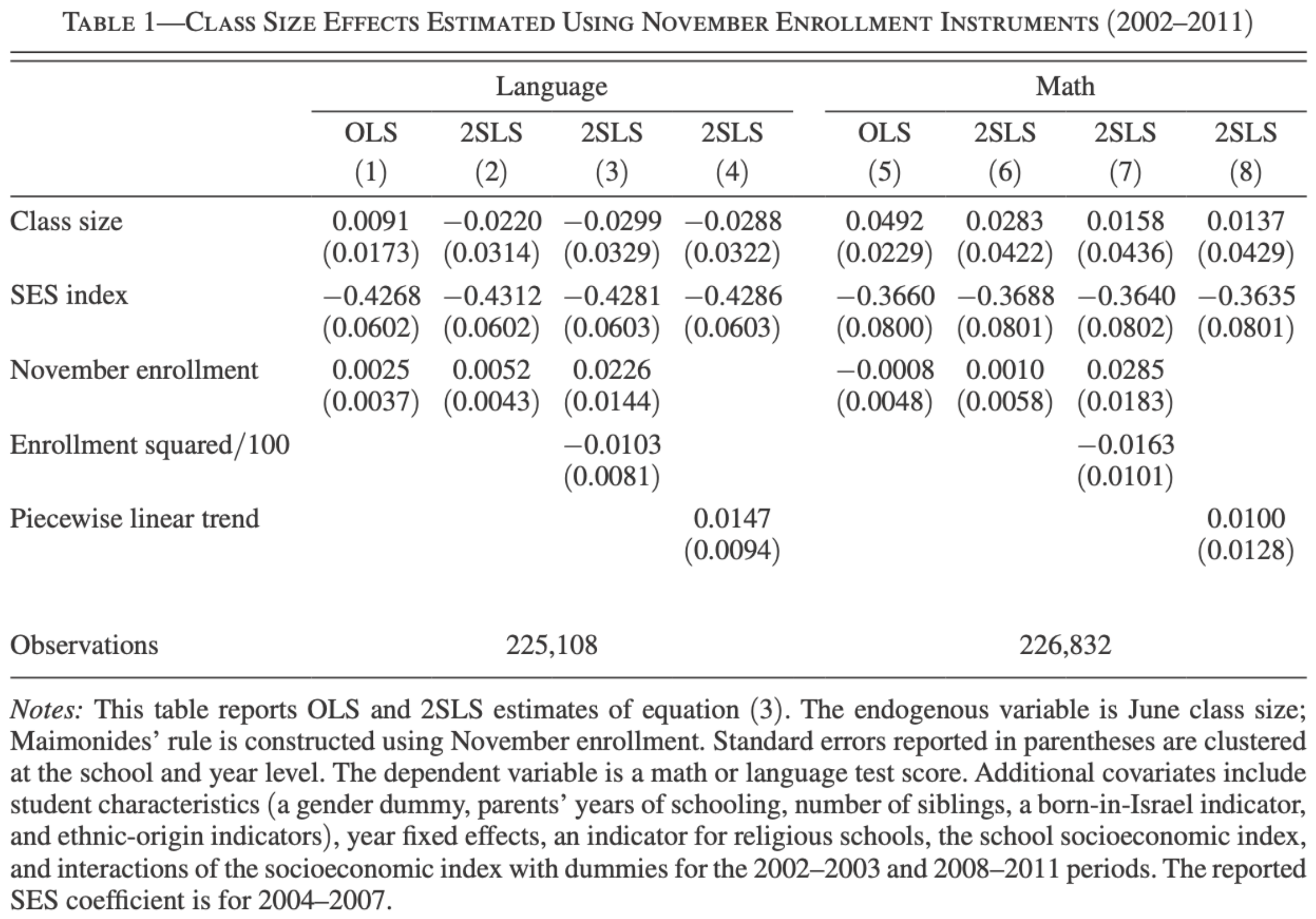
Angrist, Lavy, Leder-Luis and Shany (2019), Table 1. November enrolment.
Redux: Table 2
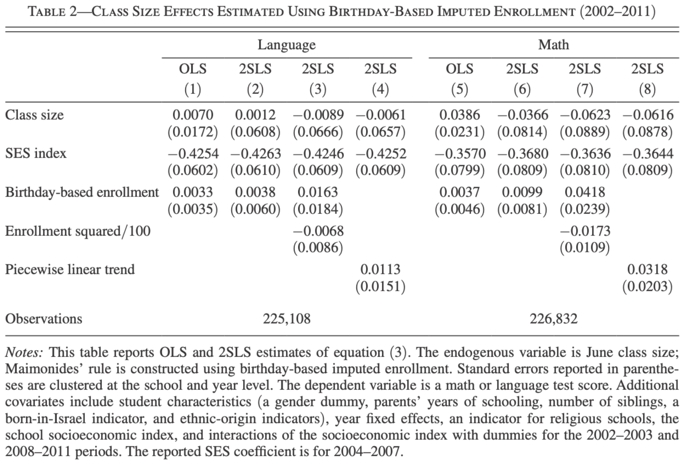
Angrist, Lavy, Leder-Luis and Shany (2019), Table 2. Birthday-based imputed enrolment.
Assessing an RD Study
- Identify the running variable, cutoff, treatment and outcome.
- Explain why potential outcomes should be continuous at the cutoff.
- Examine outcome plots, predetermined characteristics and the score distribution.
- Assess bandwidth choice, functional form and uncertainty.
- For fuzzy RD, inspect the first stage and explain exclusion and monotonicity.
- State whose effect is identified and how far the policy conclusion extends.
9. Python: generating and analysing the example
The code below constructs the same population before and after manipulation. It estimates each regression separately. Run the blocks in order. The full Python file contains the same code.
Install rdrobust and rddensity alongside NumPy, pandas, Matplotlib and statsmodels. The output paths below follow the course project. When running the file elsewhere, create the folder resources/images/week-07 or change the file names in fig.savefig() to your preferred location.
The figures are already displayed above. The code saves them without displaying a second copy in these notes.
Generate a population with a known treatment effect
Let some people change their recorded score
# People just below zero with above-average ability move across the cutoff.
# Reflecting their score puts them just above zero without creating a mass at zero.
moves = (original_score >= -0.4) & (original_score < 0) & (ability > 0)
recorded_score = original_score.copy()
recorded_score[moves] = -original_score[moves]

# Ability and the untreated outcome stay unchanged. Treatment follows the new score.
treatment_after = (recorded_score >= 0).astype(int)
outcome_after = outcome_without_treatment + 2 * treatment_after

sample = pd.DataFrame({
    "original_score": original_score,
    "recorded_score": recorded_score,
    "ability": ability,
    "moves": moves,
    "treatment_before": treatment_before,
    "treatment_after": treatment_after,
    "outcome_before": outcome_before,
    "outcome_after": outcome_after,
    "outcome_without_treatment": outcome_without_treatment
})
print("People who change their score:", int(sample["moves"].sum()))
Plot the score distribution before manipulation
# Zero is a bin boundary, so no bin crosses the treatment cutoff.
bin_edges = np.linspace(-2, 2, 41)
fig, ax = plt.subplots(figsize=(10, 5))
ax.hist(sample["original_score"], bins=bin_edges, density=True,
        color="#0072B2", edgecolor="white")
ax.axvline(0, color="black", linestyle="--", linewidth=2)
ax.set(xlabel="Original score", ylabel="Density", xlim=(-2, 2), ylim=(0, 0.46))
fig.tight_layout()
fig.savefig("resources/images/week-07/density-before.png", dpi=200)
plt.close(fig)
Plot the score distribution after manipulation, on the same axes
fig, ax = plt.subplots(figsize=(10, 5))
ax.hist(sample["recorded_score"], bins=bin_edges, density=True,
        color="#D55E00", edgecolor="white")
ax.axvline(0, color="black", linestyle="--", linewidth=2)
ax.set(xlabel="Recorded score", ylabel="Density", xlim=(-2, 2), ylim=(0, 0.46))
fig.tight_layout()
fig.savefig("resources/images/week-07/density-after.png", dpi=200)
plt.close(fig)
Calculate bin means for ability and outcomes
sample["original_bin"] = pd.cut(sample["original_score"], bin_edges, right=False)
sample["recorded_bin"] = pd.cut(sample["recorded_score"], bin_edges, right=False)
before_means = sample.groupby("original_bin", observed=True)[
    ["original_score", "ability", "outcome_before", "outcome_without_treatment"]
].mean()
after_means = sample.groupby("recorded_bin", observed=True)[
    ["recorded_score", "ability", "outcome_after", "outcome_without_treatment"]
].mean()
Show how the composition changes
fig, ax = plt.subplots(figsize=(10, 5))
ax.scatter(before_means["original_score"], before_means["ability"],
           color="#0072B2", marker="o", label="Before manipulation")
ax.scatter(after_means["recorded_score"], after_means["ability"],
           color="#D55E00", marker="^", label="After manipulation")
ax.axvline(0, color="black", linestyle="--", linewidth=2)
ax.axhline(0, color="black", linewidth=0.7)
ax.set(xlabel="Score", ylabel="Mean ability within each bin", xlim=(-1, 1))
ax.legend()
fig.tight_layout()
fig.savefig("resources/images/week-07/ability-sorting.png", dpi=200)
plt.close(fig)
Show the consequence for observed outcomes
fig, ax = plt.subplots(figsize=(10, 5))
ax.scatter(before_means["original_score"], before_means["outcome_before"],
           color="#0072B2", marker="o", label="Before manipulation")
ax.scatter(after_means["recorded_score"], after_means["outcome_after"],
           color="#D55E00", marker="^", label="After manipulation")
ax.axvline(0, color="black", linestyle="--", linewidth=2)
ax.set(xlabel="Score", ylabel="Mean observed outcome within each bin", xlim=(-1, 1))
ax.legend()
fig.tight_layout()
fig.savefig("resources/images/week-07/outcome-sorting.png", dpi=200)
plt.close(fig)
Estimate a sharp RD with familiar regression code
# Centre the score at the cutoff. Here the cutoff is already zero.
# score_right allows the slope to differ above the cutoff.
sample["score_right_before"] = sample["original_score"] * sample["treatment_before"]
sample["score_right_after"] = sample["recorded_score"] * sample["treatment_after"]
local_before = sample.loc[sample["original_score"].abs() < 0.4].copy()
local_after = sample.loc[sample["recorded_score"].abs() < 0.4].copy()

ols_before = smf.ols(
    "outcome_before ~ treatment_before + original_score + score_right_before",
    data=local_before
).fit(cov_type="HC1")
print(ols_before.summary())

ols_after = smf.ols(
    "outcome_after ~ treatment_after + recorded_score + score_right_after",
    data=local_after
).fit(cov_type="HC1")
print(ols_after.summary())
Give observations closer to zero more weight
local_before["weight"] = 1 - local_before["original_score"].abs() / 0.4
weighted_before = smf.wls(
    "outcome_before ~ treatment_before + original_score + score_right_before",
    data=local_before, weights=local_before["weight"]
).fit(cov_type="HC1")
print(weighted_before.summary())
Use rdrobust for bandwidth selection and bias-corrected inference
Use the robust bias-corrected confidence interval and p-value when interpreting the package output. Its conventional local-linear point estimate and bias-corrected estimate can differ. The bandwidth is selected separately for each sample.
rd_before = rd.rdrobust(y=sample["outcome_before"], x=sample["original_score"],
                       c=0, p=1, kernel="triangular", bwselect="mserd")
print(rd_before)
rd_after = rd.rdrobust(y=sample["outcome_after"], x=sample["recorded_score"],
                      c=0, p=1, kernel="triangular", bwselect="mserd")
print(rd_after)
Test for a density discontinuity
The hypothesis is equal limiting densities at zero. The code prints the default jackknife standard-error test statistic and its p-value explicitly, because some package versions show only settings when printing the result object.
# This is the Cattaneo-Jansson-Ma implementation of density-discontinuity testing.
density_before = density.rddensity(X=sample["original_score"], c=0)
print(density_before)
density_after = density.rddensity(X=sample["recorded_score"], c=0)
print(density_after)

# The default printout in some versions only shows the estimation settings.
# Extract the default jackknife test statistic and p-value explicitly.
print("Before: density-test statistic =", density_before.test["t_jk"])
print("Before: density-test p-value =", density_before.test["p_jk"])
print("After: density-test statistic =", density_after.test["t_jk"])
print("After: density-test p-value =", density_after.test["p_jk"])
Checking the simulation results
With seed 2026, the separate-slopes OLS regressions within 0.4 of the cutoff estimate jumps of 1.8846 before manipulation and 4.0898 after manipulation. The true treatment effect is 2 in both cases. Sampling variation explains why the first estimate is not exactly 2. The second comparison also includes the discontinuity in ability.
Automatic bandwidth selection with rdrobust gives conventional local-linear point estimates of approximately 1.951 and 4.527. These differ from the fixed-window OLS estimates because the bandwidths and weights differ. After manipulation, the package estimates an observed discontinuity that no longer has the intended causal interpretation.
Using Python for fuzzy RD
For a dataset df containing the outcome, running variable and treatment received, the same package estimates the ratio of discontinuities:
fuzzy_results = rd.rdrobust(
    y=df["outcome"],
    x=df["score"],
    c=0,
    fuzzy=df["treatment"],
    p=1,
    kernel="triangular",
    bwselect="mserd"
)
print(fuzzy_results)
Report the first-stage discontinuity as well as the fuzzy RD estimate. Read the sample and bandwidth information in the output. The official RD software documentation describes the estimation options. The density-test documentation explains the companion diagnostic.
NoteYour turn
Run the simulation. Compare the estimated jump before and after sorting with the true effect of 2. Explain why changing the bandwidth cannot repair the failure of continuity after sorting. Then change the seed and examine which conclusions persist.
References
- Jacob, R., P. Zhu, M.-A. Somers, and H. Bloom (2012). A Practical Guide to Regression Discontinuity. MDRC.
- Imbens, G. W., and T. Lemieux (2008). “Regression Discontinuity Designs: A Guide to Practice.” Journal of Econometrics 142(2): 615–635.
- Lee, D. S. (2008). “Randomized Experiments from Non-random Selection in U.S. House Elections.” Journal of Econometrics 142(2): 675–697.
- Meyersson, E. (2014). “Islamic Rule and the Empowerment of the Poor and Pious.” Econometrica 82(1): 229–269.
- Angrist, J. D., and V. Lavy (1999). “Using Maimonides’ Rule to Estimate the Effect of Class Size on Scholastic Achievement.” Quarterly Journal of Economics 114(2): 533–575.
- Angrist, J. D., V. Lavy, J. Leder-Luis, and A. Shany (2019). “Maimonides’ Rule Redux.” American Economic Review: Insights 1(3): 309–324.
- McCrary, J. (2008). “Manipulation of the Running Variable in the Regression Discontinuity Design: A Density Test.” Journal of Econometrics 142(2): 698–714.
- Cattaneo, M. D., M. Jansson, and X. Ma (2020). “Simple Local Polynomial Density Estimators.” Journal of the American Statistical Association 115(531): 1449–1455.
- Calonico, S., M. D. Cattaneo, and R. Titiunik (2014). “Robust Nonparametric Confidence Intervals for Regression-Discontinuity Designs.” Econometrica 82(6): 2295–2326.
- Calonico, S., M. D. Cattaneo, M. H. Farrell, and R. Titiunik (2019). “Regression Discontinuity Designs Using Covariates.” Review of Economics and Statistics 101(3): 442–451.
- Imbens, G., and K. Kalyanaraman (2012). “Optimal Bandwidth Choice for the Regression Discontinuity Estimator.” Review of Economic Studies 79(3): 933–959.
- Gelman, A., and G. Imbens (2019). “Why High-Order Polynomials Should Not Be Used in Regression Discontinuity Designs.” Journal of Business & Economic Statistics 37(3): 447–456.
- Lee, D. S., and T. Lemieux (2010). “Regression Discontinuity Designs in Economics.” Journal of Economic Literature 48(2): 281–355. Advanced reading.