Regression Discontinuity Designs
PP5001 · Week 7 · Martinmas 2026
Sharp Regression Discontinuity
Let X_i be the running variable and x_0 the known cutoff:
D_i=\begin{cases}1 & \text{if }X_i\ge x_0,\\0 & \text{if }X_i<x_0.\end{cases}
Assignment is deterministic: once we know X_i, we know D_i.
Treatment changes discontinuously at x_0. The running variable itself may change by an arbitrarily small amount while treatment changes from 0 to 1.
Sharp Discontinuity
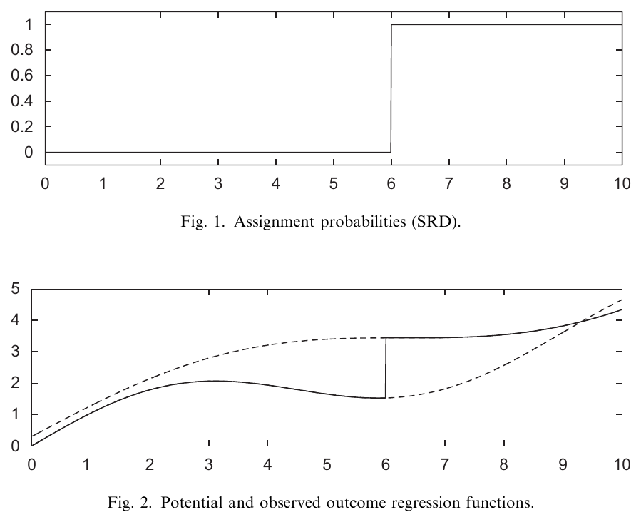
Imbens and Lemieux (2008), Figures 1–2.
The Causal Effect at the Cutoff
Using our potential-outcome notation, define
\rho=E\left[Y_i^1-Y_i^0\mid X_i=x_0\right].
The observed outcome is
Y_i=D_iY_i^1+\left(1-D_i\right)Y_i^0.
To the right of the cutoff we observe treated outcomes. To the left we observe untreated outcomes.
With a continuously distributed score, identification uses the limiting conditional means as we approach x_0 from each side.
The Continuity Assumption
For each potential outcome, the conditional mean approaches the same value from either side of the cutoff:
\lim_{x\uparrow x_0}E\left[Y_i^0\mid X_i=x\right] =\lim_{x\downarrow x_0}E\left[Y_i^0\mid X_i=x\right] =E\left[Y_i^0\mid X_i=x_0\right].
\lim_{x\uparrow x_0}E\left[Y_i^1\mid X_i=x\right] =\lim_{x\downarrow x_0}E\left[Y_i^1\mid X_i=x\right] =E\left[Y_i^1\mid X_i=x_0\right].
Average outcomes under either treatment state would change smoothly as we cross the cutoff.
The two potential-outcome means can differ from one another. That difference at x_0 is the treatment effect.
Deriving the Sharp RD Effect
Immediately to the right, D_i=1. By continuity,
\lim_{x\downarrow x_0}E\left[Y_i\mid X_i=x\right] =E\left[Y_i^1\mid X_i=x_0\right].
Immediately to the left, D_i=0. By continuity,
\lim_{x\uparrow x_0}E\left[Y_i\mid X_i=x\right] =E\left[Y_i^0\mid X_i=x_0\right].
Subtracting gives
\rho=\lim_{x\downarrow x_0}E\left[Y_i\mid X_i=x\right] -\lim_{x\uparrow x_0}E\left[Y_i\mid X_i=x\right].
Lee (2008): Elections and Incumbency
Lee studies US House elections and the effect of winning office on subsequent electoral success.
- Running variable: the Democratic winning margin in the current election.
- Cutoff: a margin of zero.
- Treatment: a Democratic victory in the current election.
- Outcomes: subsequent candidacy, vote share, and victory.
Why should narrow winners and narrow losers be informative about the effect of incumbency?
Lee: Subsequent Democratic Vote Share
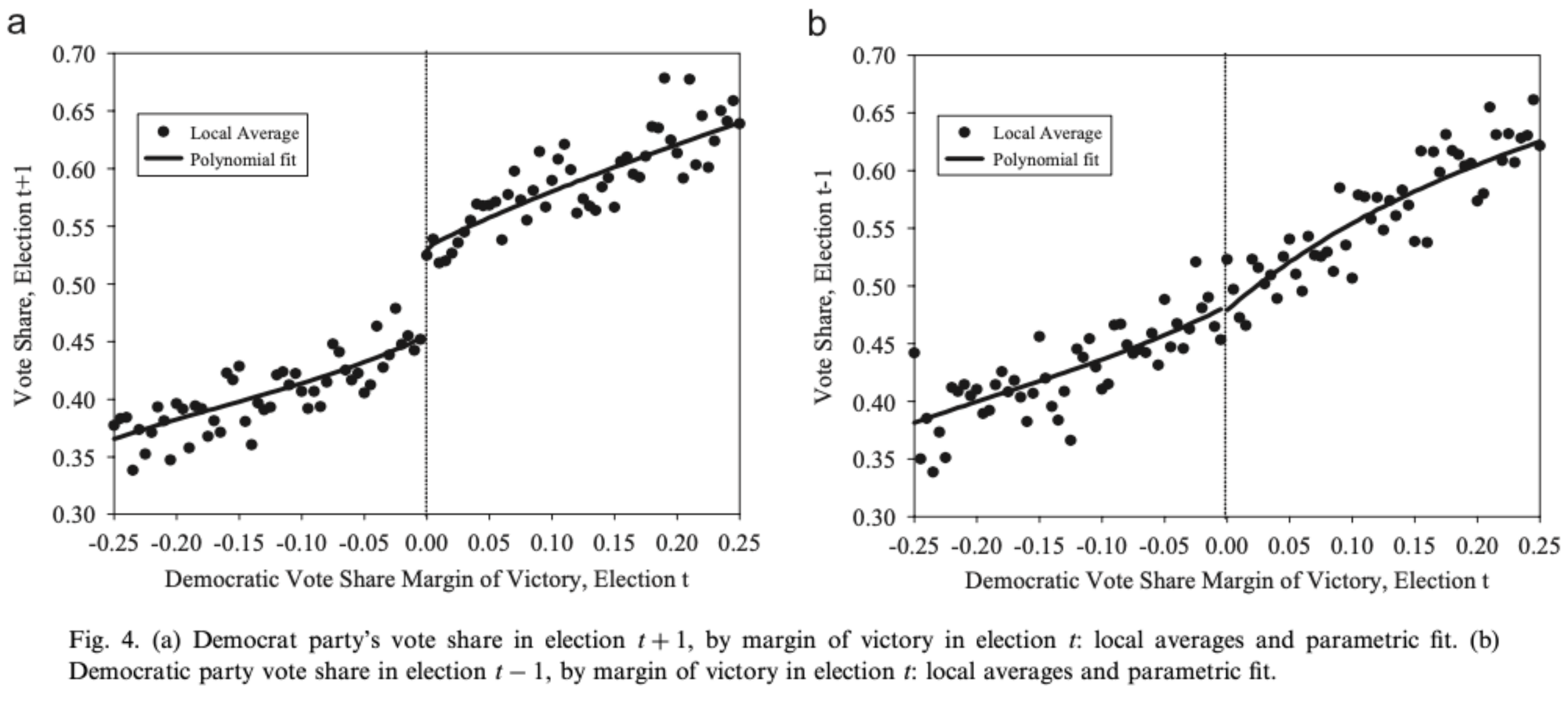
Lee (2008), Figure 4.
RD as a Regression
Centre the running variable: R_i=X_i-x_0.
Suppose, locally,
E\left[Y_i^0\mid X_i\right]=\beta_0+\beta_1R_i,\qquad Y_i^1=Y_i^0+\rho.
Then
Y_i=\beta_0+\beta_1R_i+\rho D_i+\epsilon_i.
Here \epsilon_i=Y_i^0-E\left[Y_i^0\mid X_i\right] is the disturbance: the difference between an individual’s untreated outcome and its conditional mean. Thus E\left[\epsilon_i\mid X_i\right]=0.
At R_i=0, the fitted untreated outcome is \beta_0 and the fitted treated outcome is \beta_0+\rho.
The difference between the intercepts is the treatment effect at the cutoff.
Allowing Different Slopes
Allow the relationship between the score and the outcome to differ on the two sides:
Y_i=\beta_0+\rho D_i+\beta_1R_i+\gamma_1D_iR_i+\epsilon_i.
- Below the cutoff: intercept \beta_0, slope \beta_1.
- Above the cutoff: intercept \beta_0+\rho, slope \beta_1+\gamma_1.
Because R_i=0 at the cutoff, the interaction contributes zero there. The jump remains \rho.
Polynomial Regression
If the conditional mean is curved, we can allow powers of the centred score:
Y_i=\beta_0+\rho D_i+ \sum_{j=1}^{p}\beta_jR_i^j+ \sum_{j=1}^{p}\gamma_jD_iR_i^j+\epsilon_i.
The two sums allow different shapes on either side of the cutoff.
At R_i=0, all the terms in those sums are zero, so \rho remains the jump.
A high-order polynomial over a wide range can fit poorly near the cutoff and confuse curvature with a discontinuity.
Local Regression and Bandwidth
Use observations within a bandwidth h of the cutoff: -h<R_i<h.
Fit a separate line on each side and compare the fitted values at R_i=0.
With a cutoff of 50, h=10 uses scores between 40 and 60. With h=5, use 45 to 55.
- A smaller bandwidth gives a more local comparison with fewer observations.
- A wider bandwidth provides more observations, but fitting a simple function over a wider range can introduce approximation bias.
Kernel Weights and Local Linear Regression
A kernel assigns weights according to distance from the cutoff.
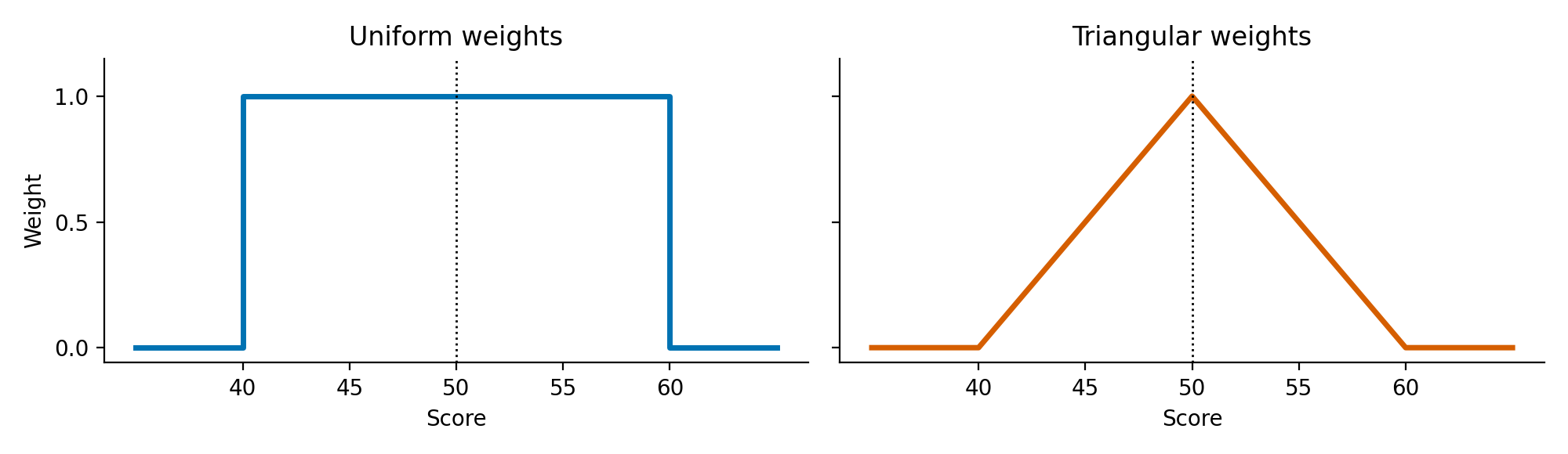
With triangular weights, w_i=1-|R_i|/h inside the bandwidth and zero outside it.
Estimate by weighted least squares:
\min_{\beta_0,\rho,\beta_1,\gamma_1}\sum_i w_i\left(Y_i-\beta_0-\rho D_i-\beta_1R_i-\gamma_1D_iR_i\right)^2.
Bandwidth Choice and Inference
A data-driven bandwidth balances squared bias and variance: mean squared error.
At an MSE-optimal bandwidth, approximation bias can still be large enough to matter for confidence intervals.
Robust bias-corrected inference estimates that bias and accounts for the uncertainty from estimating the correction.
The rdrobust package implements bandwidth selection, local polynomial estimation, and robust bias-corrected inference.
An Illustration
Generate independent scores and disturbances:
X_i^*\sim U\left(-2,2\right),\qquad A_i,u_i\sim N\left(0,1\right).
Y_i^0=10+0.5X_i^*+2A_i+u_i,\qquad Y_i^1=Y_i^0+2.
Initially X_i=X_i^* and D_i=1\left(X_i\ge0\right). The true effect is 2.
Now let people with -0.4\le X_i^*<0 and A_i>0 report X_i=-X_i^*.
Their ability and untreated outcomes stay the same. Crossing zero gives them treatment. Everyone else keeps their original score.
Before and After Manipulation
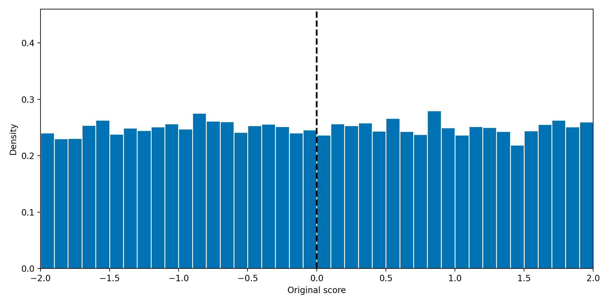
Before
After
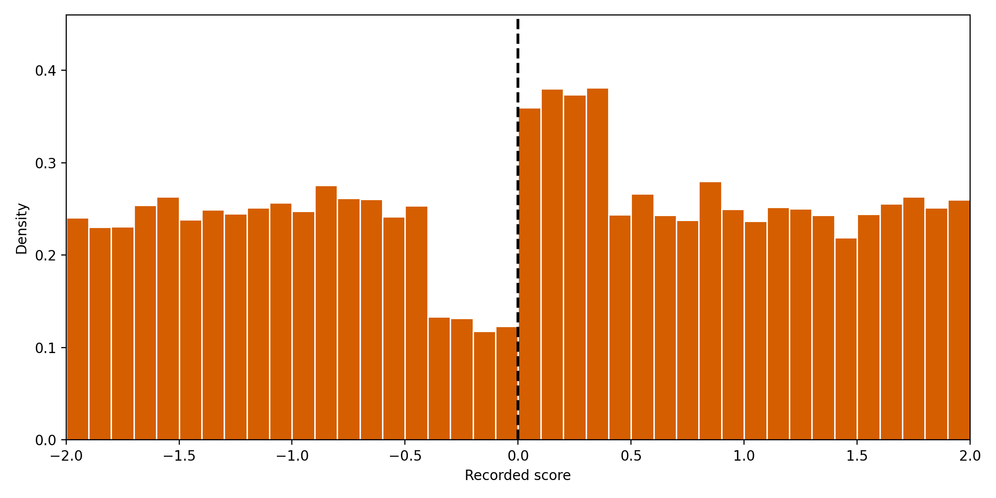
Same people, bins, and vertical scale. Only the recorded scores and resulting treatment change.
The Composition of the Groups Changes
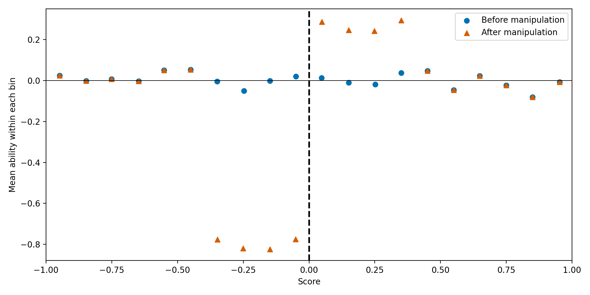
Circles: before manipulation. Triangles: after manipulation. Each point is a bin mean.
The Outcome Jump Changes Too
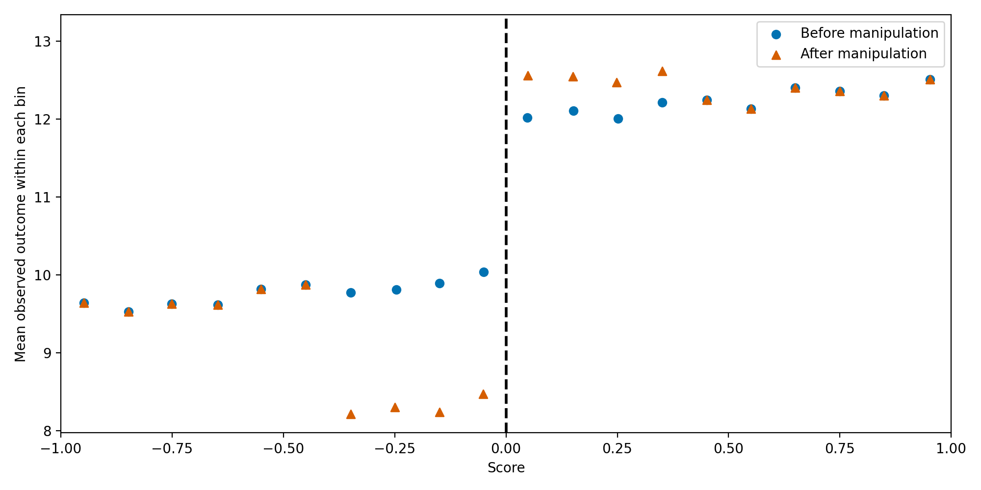
The true treatment effect remains 2 for every person.
What Does the Density Test Ask?
Let f_X\left(x\right) denote the density of the recorded running variable.
The null hypothesis is
H_0:\quad\lim_{x\uparrow x_0} f_X\left(x\right) =\lim_{x\downarrow x_0}f_X\left(x\right).
A histogram illustrates how observations are distributed. The test estimates the density on each side and assesses the uncertainty in the estimated difference.
The question concerns the number of observations near the cutoff, rather than their average outcome.
How the Cattaneo–Jansson–Ma Test Works
- Construct the empirical cumulative distribution: the proportion of observations with a score at or below each value.
- Fit local polynomials to this distribution on each side of the cutoff, using nearby observations.
- The slope of each fitted curve at the cutoff estimates the density on that side.
- Test whether the difference between the two estimated densities is zero, allowing for sampling uncertainty and smoothing bias.
The test uses individual observations, with a selected bandwidth and kernel weights. Histogram bins are used only for our descriptive graph.
Density-Test Results and Interpretation
| Recorded score | Test statistic | p-value |
|---|---|---|
| Before manipulation | −0.697 | 0.486 |
| After manipulation | 6.205 | <0.001 |
Cattaneo–Jansson–Ma test, 20,000 observations, default bandwidth selection.
- Reject continuity: investigate sorting, recording practices and institutional rules.
- Do not reject: no statistically detectable density jump. The test’s precision matters.
Combine this evidence with predetermined-characteristic checks and the assignment process. Some forms of sorting can leave the density smooth.
Sorting and Identification
For discussion
In the simulation, explain why the outcome jump changes even though the treatment effect stays at 2.
What can a researcher learn from the score distribution when ability is unobserved?
What further evidence would you seek?
Meyersson: Question and Data
For discussion
Explain the policy question, the unit of observation, and how the 1994 municipal elections are linked to the 2000 census.
Define the main educational outcome and the population it describes.
Why might municipalities with Islamic and secular mayors differ even without a causal effect of the mayor?
Meyersson: The Study and Assignment Rule
Does electing an Islamic mayor affect educational attainment?
The study links 1994 Turkish municipal elections with the 2000 census. A main outcome is high-school completion among women aged 15–20 in 2000.
The running variable is
X_i=\text{largest Islamic party vote share}_i-\text{largest secular party vote share}_i.
An Islamic party wins when its margin is positive. The cutoff is zero.
Compare municipalities where it narrowly won with those where it narrowly lost.
Meyersson: Identification Strategy
For discussion
Define the running variable, cutoff, treatment and comparison.
Explain why the cutoff is zero rather than a 50 percent vote share.
State the continuity assumption in terms of potential educational outcomes.
Discuss a plausible threat to identification and explain which municipalities the estimated effect describes.
Meyersson: Figure 4
For discussion
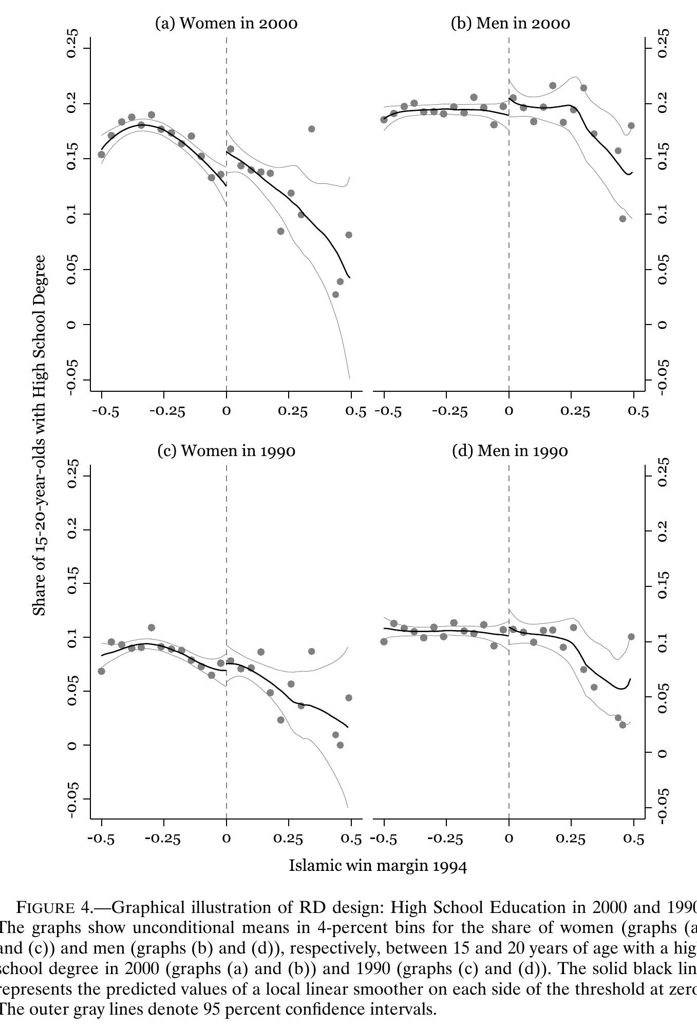
Meyersson (2014), Figure 4. High school education in 2000 and 1990.
Meyersson: Table II, Panel A
For discussion
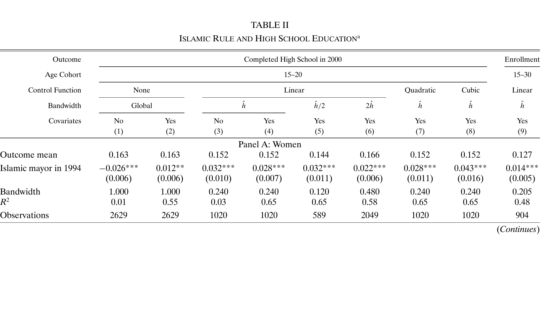
Meyersson (2014), Table II. Women.
Interpreting the Policy Effect
The comparison identifies the effect of electing an Islamic mayor in municipalities near the electoral threshold.
That treatment changes a bundle of policies, practices and political representation.
For discussion: How far can the results distinguish the mechanisms through which education changes? To which other municipalities, elections or policy reforms would you apply the findings?
Fuzzy Discontinuity
Crossing the cutoff changes treatment probability without determining treatment completely.
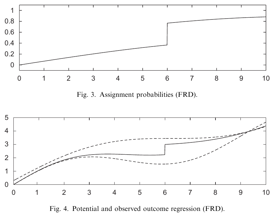
Imbens and Lemieux (2008), Figures 3–4.
The Fuzzy RD Estimand
Divide the outcome discontinuity by the treatment discontinuity:
\rho_{FRD}=\frac{ \lim_{x\downarrow x_0}E\left[Y_i\mid X_i=x\right]-\lim_{x\uparrow x_0}E\left[Y_i\mid X_i=x\right] }{ \lim_{x\downarrow x_0}E\left[D_i\mid X_i=x\right]-\lim_{x\uparrow x_0}E\left[D_i\mid X_i=x\right] }.
This is a local Wald ratio:
\frac{\text{reduced-form jump}}{\text{first-stage jump}}.
The denominator must be nonzero and estimated with sufficient precision.
What Makes the Fuzzy RD Ratio Causal?
For a binary treatment, the interpretation is a LATE at the cutoff for people whose treatment changes when eligibility changes.
We need:
- Continuity of potential outcomes and treatment behaviour through the cutoff, apart from the eligibility change.
- A nonzero first-stage discontinuity.
- Exclusion: eligibility affects the outcome through treatment.
- Monotonicity: eligibility changes treatment in the same direction for everyone at the cutoff.
Retain the well-defined-treatment and no-interference assumptions.
Fuzzy RD as Two-Stage Least Squares
Set R_i=X_i-x_0 and Z_i=1\left(R_i\ge0\right). Locally, write the first stage as
D_i=\pi_0+\pi_1Z_i+\pi_2R_i+\pi_3Z_iR_i+v_i.
The outcome equation is
Y_i=\beta_0+\rho D_i+\beta_1R_i+\gamma_1Z_iR_i+\epsilon_i.
Use Z_i as the excluded instrument for D_i.
Include R_i and Z_iR_i as controls in both equations. They allow separate slopes on the two sides.
Report the first-stage jump. A weak jump creates the denominator problem from Week 5.
Angrist and Lavy: Question and Data
For discussion
Explain the class-size policy question, the data and the outcomes.
Describe Maimonides’ rule and illustrate what happens to predicted class size when enrolment rises from 40 to 41.
Why might an OLS relationship between class size and achievement give a misleading estimate of the causal effect?
Angrist and Lavy (1999): Maimonides’ Rule
The rule limits classes to 40 pupils. As grade enrolment crosses a multiple of 40, the implied number of classes increases.
For enrolment e, predicted class size is
m\left(e\right)=\frac{e}{\lfloor\left(e-1\right)/40\rfloor+1}.
For example, 40 pupils imply one class of 40. With 41 pupils, the rule implies two classes averaging 20.5.
Actual class size does not follow the rule perfectly, creating a fuzzy design.
Angrist and Lavy: Identification Strategy
For discussion
Use the class-size and achievement graphs to explain the first stage and reduced form.
Explain why this is a fuzzy design.
Discuss relevance, exclusion, local comparability and the direction of the class-size change induced by the rule.
Could another school input change at the enrolment threshold?
Actual and Predicted Class Size
For discussion
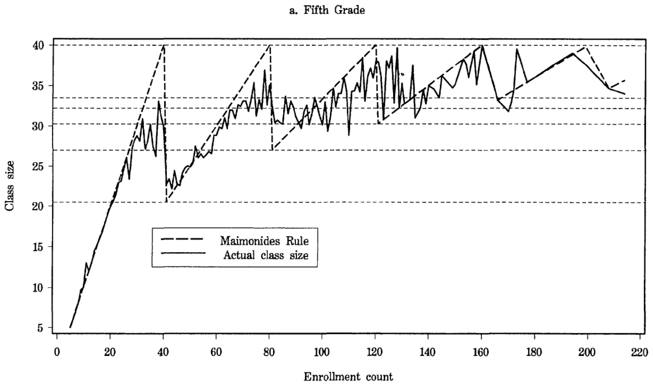
Angrist and Lavy (1999), class-size figure from the original slides.
The Reduced Form
For discussion
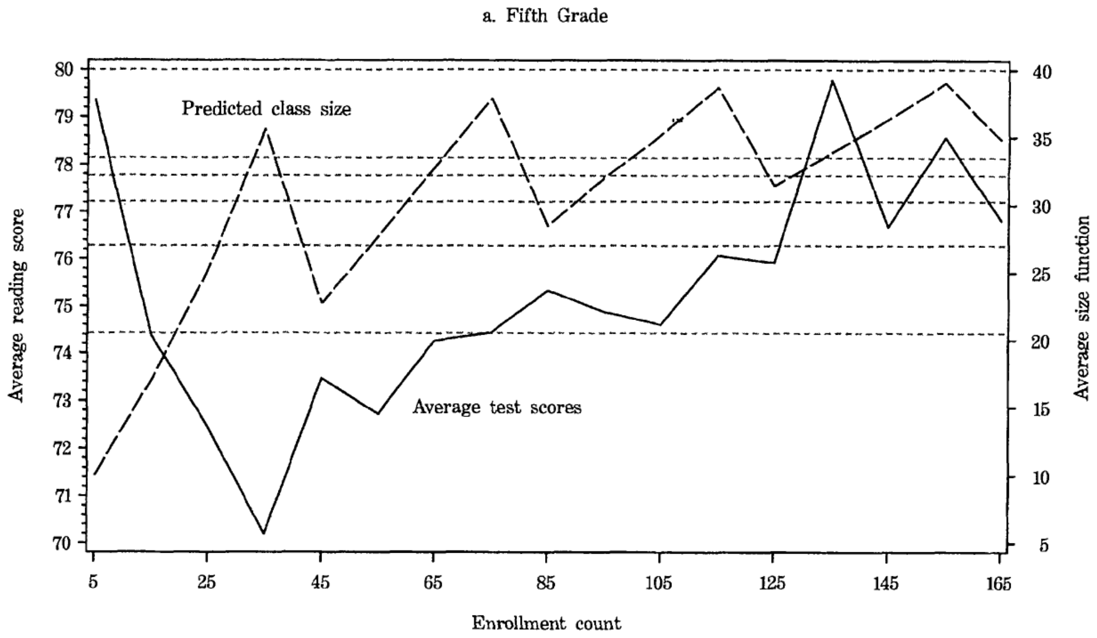
Angrist and Lavy (1999), achievement and enrolment figure from the original slides.
Angrist and Lavy: Table IV
For discussion
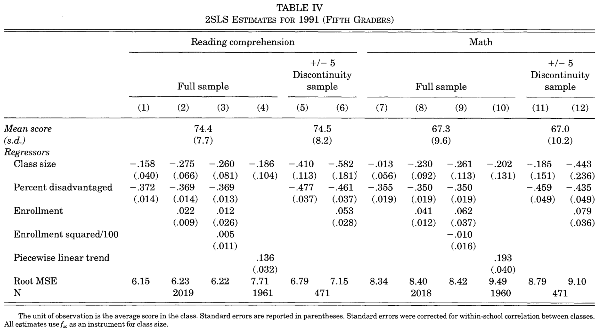
Angrist and Lavy (1999), Table IV. IV results.
Maimonides’ Rule Redux
For discussion
Explain what the newer data allow the authors to examine and why manipulation of reported enrolment matters.
Describe the alternative enrolment measure based on birthdays.
Use Table 2 to discuss the first stage, achievement estimates and uncertainty.
How does the follow-up affect your interpretation of the original findings?
Maimonides’ Rule Redux (2019)
The follow-up uses much larger Israeli samples from 2002–2011.
- The rule still predicts class size, but the achievement estimates are close to zero.
- Reported enrolment shows manipulation near the thresholds.
- An alternative instrument uses enrolment imputed from birthdays.
Compare the estimates and confidence intervals with the original findings. For class size, interpret the effect per pupil, rather than as a binary-treatment LATE.
What does the follow-up teach us about the original design and its policy interpretation?
Redux: Table 2
For discussion
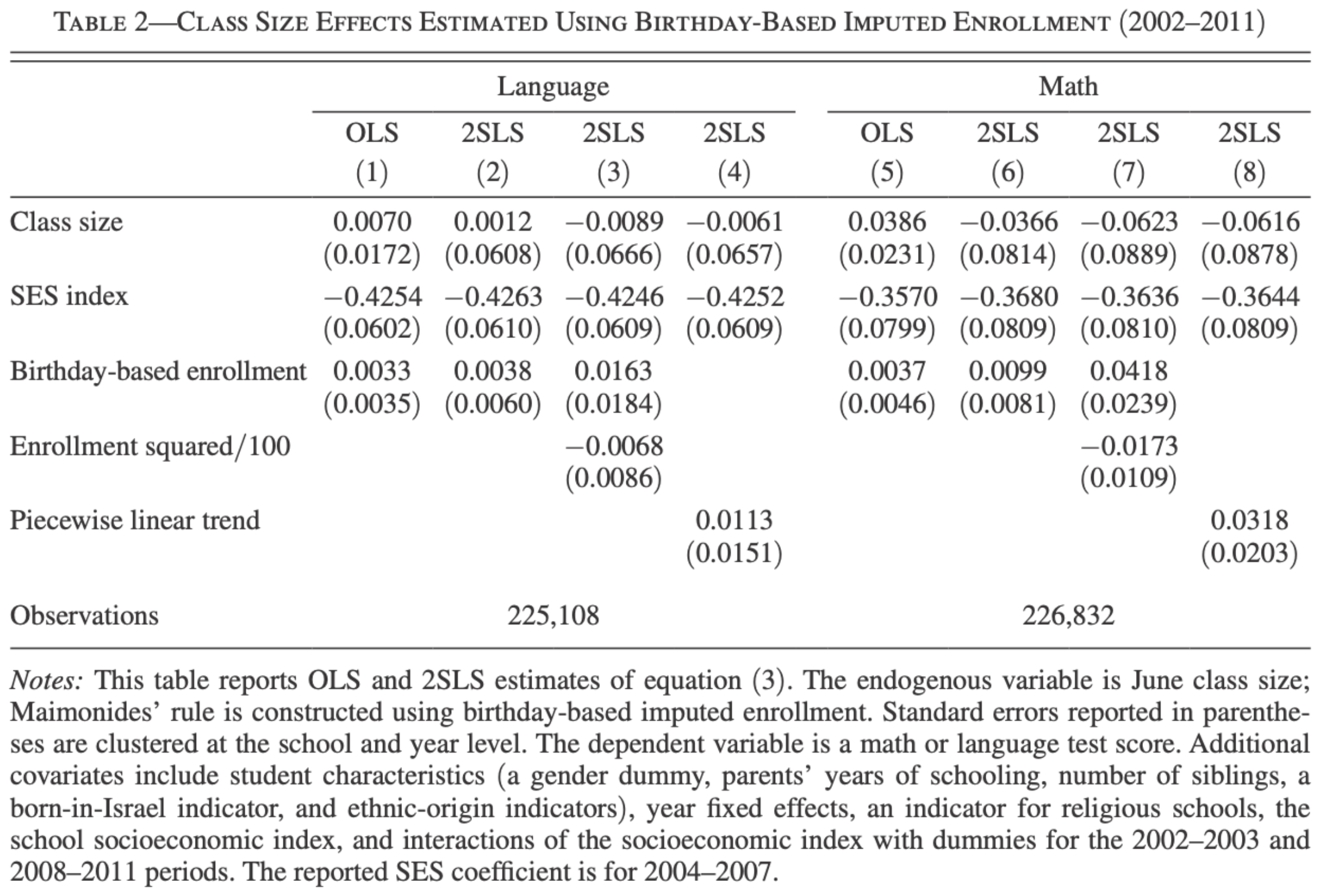
Angrist, Lavy, Leder-Luis and Shany (2019), Table 2. Birthday-based imputed enrolment.
References
- Jacob, R., P. Zhu, M.-A. Somers, and H. Bloom (2012). A Practical Guide to Regression Discontinuity. MDRC.
- Imbens, G. W., and T. Lemieux (2008). “Regression Discontinuity Designs: A Guide to Practice.” Journal of Econometrics 142(2): 615–635.
- Lee, D. S. (2008). “Randomized Experiments from Non-random Selection in U.S. House Elections.” Journal of Econometrics 142(2): 675–697.
- Meyersson, E. (2014). “Islamic Rule and the Empowerment of the Poor and Pious.” Econometrica 82(1): 229–269.
- Angrist, J. D., and V. Lavy (1999). “Using Maimonides’ Rule to Estimate the Effect of Class Size on Scholastic Achievement.” Quarterly Journal of Economics 114(2): 533–575.
- Angrist, J. D., V. Lavy, J. Leder-Luis, and A. Shany (2019). “Maimonides’ Rule Redux.” American Economic Review: Insights 1(3): 309–324.
- McCrary, J. (2008). “Manipulation of the Running Variable in the Regression Discontinuity Design: A Density Test.” Journal of Econometrics 142(2): 698–714.
- Cattaneo, M. D., M. Jansson, and X. Ma (2020). “Simple Local Polynomial Density Estimators.” Journal of the American Statistical Association 115(531): 1449–1455.
- Calonico, S., M. D. Cattaneo, and R. Titiunik (2014). “Robust Nonparametric Confidence Intervals for Regression-Discontinuity Designs.” Econometrica 82(6): 2295–2326.
- Calonico, S., M. D. Cattaneo, M. H. Farrell, and R. Titiunik (2019). “Regression Discontinuity Designs Using Covariates.” Review of Economics and Statistics 101(3): 442–451.
- Imbens, G., and K. Kalyanaraman (2012). “Optimal Bandwidth Choice for the Regression Discontinuity Estimator.” Review of Economic Studies 79(3): 933–959.
- Gelman, A., and G. Imbens (2019). “Why High-Order Polynomials Should Not Be Used in Regression Discontinuity Designs.” Journal of Business & Economic Statistics 37(3): 447–456.
- Lee, D. S., and T. Lemieux (2010). “Regression Discontinuity Designs in Economics.” Journal of Economic Literature 48(2): 281–355. Advanced reading.