Week 11: Synthetic Controls

California tobacco control and German reunification · PP5001 · Martinmas 2026

Post-class exercise · Class slides · Slides PDF · Notes PDF

Learning Objectives

By the end of this session, you should be able to:

• Explain how a weighted combination of untreated units supplies a counterfactual for one treated unit.
• Distinguish donor weights from the weights given to different predictors.
• Assess donor selection, pre-treatment fit, and the assumptions needed for a causal interpretation.
• Interpret treatment-effect paths, placebo comparisons, and sensitivity checks.
• Evaluate the evidence on California tobacco control and German reunification.

Reading

Read the notes and the two empirical papers before class. Read the German reunification paper alongside its erratum. The papers are available in Moodle.

• Abadie, Diamond, and Hainmueller (2010), California tobacco control, JASA.
• Abadie, Diamond, and Hainmueller (2015), German reunification, AJPS, with the 2025 erratum.

Textbook guide: The Remix, Chapter 11 and The Effect, Section 22.2.1.

Advanced reading: Abadie (2021), Journal of Economic Literature.

Choosing a Comparison Group

One of the fundamental issues with difference-in-differences is choosing the right control group.

Synthetic control uses pre-treatment data to choose weights for untreated units so that their weighted average resembles the treated unit.

The resulting synthetic control supplies an estimated counterfactual path after treatment.

A state or country may have no single convincing counterpart. Several untreated units can contribute different features of its pre-treatment experience. A long pre-treatment period helps us assess whether that combination tracks the treated unit through changes in economic conditions.

The Counterfactual Problem

For treated unit 1, the effect at time t is

\tau_{1t}=Y_{1t}^{1}-Y_{1t}^{0}.

After treatment begins, we observe Y_{1t}=Y_{1t}^{1}.

We need Y_{1t}^{0}: the outcome that would have occurred without treatment.

The superscripts retain our treatment-state notation. Here treatment means exposure to the intervention from its start date onward. We follow one treated unit over time, so the effect can change with time since the intervention.

From Difference-in-Differences

A simple DiD comparison is

\widehat\tau^{\mathrm{DiD}}= \left(Y_{1,\mathrm{post}}-Y_{1,\mathrm{pre}}\right) -\left(\bar Y_{C,\mathrm{post}}-\bar Y_{C,\mathrm{pre}}\right).

The choice of controls determines \bar Y_{C,t}.

We could use one comparison unit, a simple average, a population-weighted average, or weights selected using pre-treatment data.

DiD allows a persistent difference in levels under parallel trends. Standard synthetic control seeks a weighted combination that closely reproduces pre-treatment outcome levels as well as relevant predictors. We then interpret the post-treatment gap relative to that fitted comparison.

California: Figure 1

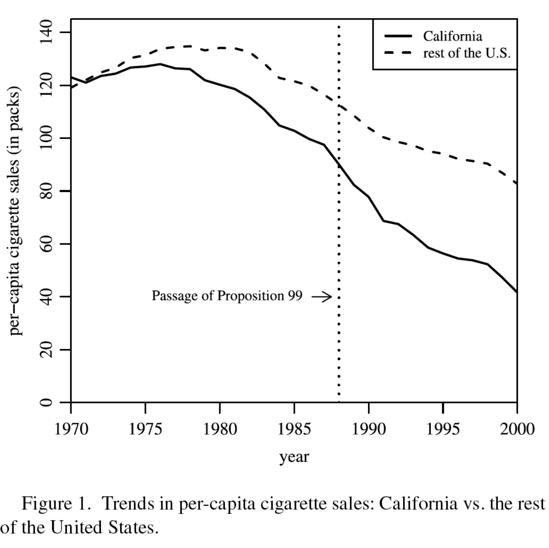
Abadie, Diamond, and Hainmueller (2010), Figure 1.

For discussion: How well does the rest of the United States track California before the intervention? What would you want a better comparison to reproduce?

The Basic Idea

Donor units remain untreated, so Y_{jt}=Y_{jt}^{0} for j=2,\ldots,J+1.

Construct the counterfactual:

\widehat Y_{1t}^{0}=\sum_{j=2}^{J+1}w_jY_{jt}.

Then estimate the effect:

\widehat\tau_{1t}=Y_{1t}-\widehat Y_{1t}^{0}.

How do we choose the donor weights w_j?

For example, a synthetic unit might put 0.6 on one donor and 0.4 on another. Its outcome in each year is 0.6 times the first donor’s outcome plus 0.4 times the second’s. The weights are chosen before treatment and held fixed afterward.

Setup

• One treated unit, indexed by 1.
• J untreated units in the donor pool.
• A balanced panel observed for T periods.
• T_0 pre-treatment periods, with treatment beginning in period T_0+1.
• T_1=T-T_0 post-treatment periods.

The donor pool is a substantive choice. Include units whose outcomes could plausibly inform the untreated path, and consider whether other policies or spillovers affect them. Stable definitions and consistent measurement across units and years matter.

Donor Weights

The standard method imposes

w_j\ge0\quad\text{for every donor }j,

and

\sum_{j=2}^{J+1}w_j=1.

The synthetic unit is a weighted average of observed donor units.

Some donors can receive zero weight.

A weight of 0.25 means that donor contributes one quarter of the synthetic outcome in every period. These restrictions keep the synthetic unit within the range of combinations available from the donor pool. The weights describe the comparison, not treatment effects for the donor units.

Predictors and Pre-Treatment Outcomes

Let X_{hj} be predictor h for unit j, for h=1,\ldots,K.

Predictors can include:

• Observable characteristics measured before treatment.
• Selected pre-treatment outcomes.
• Pre-treatment averages of outcomes.

The synthetic value of predictor h is \sum_{j=2}^{J+1}w_jX_{hj}.

The predictors should help explain the outcome. Their measurement must precede the intervention. Examples in the two applications include past cigarette sales or GDP, alongside relevant economic and demographic characteristics.

Choosing the Donor Weights

Choose w_2,\ldots,w_{J+1} to minimize

\sum_{h=1}^{K}v_h \left(X_{h1}-\sum_{j=2}^{J+1}w_jX_{hj}\right)^2,

subject to w_j\ge0 and \sum_{j=2}^{J+1}w_j=1.

The expression in parentheses is the treated–synthetic difference for predictor h.

v_h determines how much that predictor contributes to the criterion.

This is the diagonal-predictor-weight version of the criterion in the original slides. Squaring makes positive and negative discrepancies contribute to the loss. A larger predictor weight makes a given discrepancy more costly. The same donor weights must jointly match all the predictors.

Two Different Sets of Weights

Donor weights w_j: how much each state or country contributes to the synthetic unit.

Predictor weights v_h: how much each predictor matters when choosing that combination.

Large v_h places more emphasis on matching predictor h.

The choice of predictor weights can change the donor weights.

The matrix called V in the papers collects the predictor weights. With a diagonal V, its diagonal entries are the v weights shown here. We use the scalar expression so that we can see each squared difference and its contribution directly.

Choosing Predictor Weights

One option is v_h=1/\sigma_h^2, where \sigma_h^2 is the variance of predictor h across units.

Another is to choose predictor weights that produce good pre-treatment outcome predictions.

We can assess prediction using a training period and a later validation period, both before treatment.

Inverse-variance weights put predictors measured on different scales on a more comparable footing. A predictor with zero variance supplies no distinguishing information and cannot be scaled this way.

For a candidate set of predictor weights v, let w_j^*(v) be the fitted donor weights. One criterion for selecting v is pre-treatment mean squared prediction error:

\frac{1}{T_0}\sum_{t=1}^{T_0} \left(Y_{1t}-\sum_{j=2}^{J+1}w_j^*(v)Y_{jt}\right)^2.

The calculation has two steps: find donor weights for a candidate set of predictor weights, then evaluate how well the resulting synthetic outcome predicts the treated unit. Repeat with other predictor weights.

For validation, choose donor weights using an earlier pre-treatment period and evaluate their predictions in a later pre-treatment period. This reveals whether a close training fit carries into periods not used to fit those donor weights. Choices about training, validation, and final fitting should be reported.

How Many Pre-Treatment Outcomes?

• Too few periods may miss important differences in outcome paths.
• Matching many noisy outcomes can fit transitory fluctuations.
• Using every lag as a separate predictor can make additional covariates redundant in common fitting procedures.
• Compare reasonable predictor sets and pre-treatment windows.

Your source slides cite Kaul et al. (2022) on using all pre-intervention outcomes together with covariates. The practical lesson is to explain the predictor choice and examine sensitivity. Averages or selected lags can summarize longer histories. See the advanced references for the technical argument.

Geometry of Synthetic Control

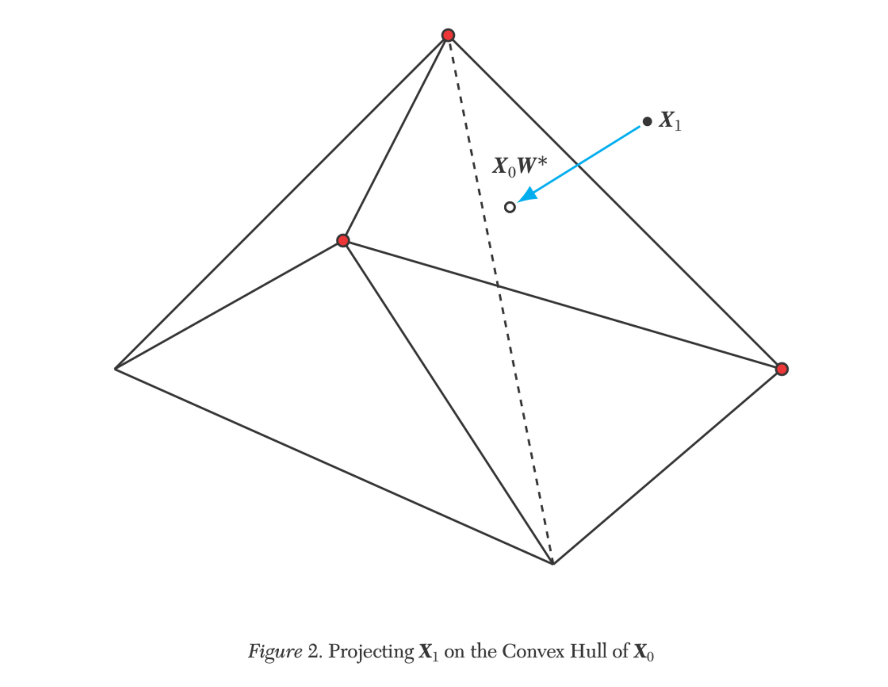
Abadie (2021), illustration from the original lecture slides.

For discussion: What combinations of donor units are available under nonnegative weights that sum to one?

The convex hull is the set of all weighted averages available under these restrictions. Exact predictor balance may be possible when the treated unit lies inside it. Outside it, the method must accept discrepancies.

Synthetic Control and OLS Weights

The regression comparison used in the German application has implied donor weights that sum to one because the regression includes an intercept.

Those weights can be negative.

Those weights allow extrapolation beyond the donor pool.

Synthetic control restricts the fitted comparison to weighted averages of the donors.

A close fit should be assessed alongside the weights that produce it.

Negative weights permit combinations such as 1.5 times one country minus 0.5 times another. The resulting counterfactual may lie beyond the observed donor outcomes. Whether that extrapolation is credible requires substantive judgment. The German application compares the two sets of weights directly.

From Fit to a Causal Interpretation

The donor combination must continue to approximate the treated unit’s untreated outcome after the intervention.

That requires attention to:

• Stable relationships between treated and donor outcomes.
• No anticipation during the fitting period.
• Untreated donors and limited spillovers.
• Other shocks unique to the treated unit at the intervention date.

Good pre-treatment fit supports the proposed comparison. Its usefulness depends on how the outcome is generated and whether that relationship persists. A treatment-date shock affecting only the treated unit could also produce a post-treatment gap. A long pre-treatment history helps us examine stability, but the missing untreated path remains unobserved.

The Gap

Using the fitted donor weights w_j^*, define

g_{1t}=Y_{1t}-\sum_{j=2}^{J+1}w_j^*Y_{jt}.

Before treatment, the gap measures fit.

After treatment,

g_{1t}=\widehat\tau_{1t}.

Interpret the gap in the units of the outcome.

A plot of the two outcome paths shows the size and movement of the outcome itself. A gap plot makes deviations easier to see. In this section, lower-case g denotes a gap, whereas in Week 10 it indexed an adoption cohort.

Why Inference Is Difficult

These applications have:

• One treated state or country.
• One intervention date.
• Outcomes related across years.
• A particular set of potential comparison units.

We need to assess how unusual the treated unit’s gap is.

Counting the number of annual observations as if each were an independent policy intervention would overstate the amount of independent information. The papers use placebo comparisons to examine whether similarly large gaps appear for untreated units.

In-Space Placebos

1. Treat a donor unit as if it received the intervention at the same date.
2. Fit a synthetic control for that unit from the other untreated donors.
3. Calculate its pre- and post-treatment gaps.
4. Repeat for the remaining donors.
5. Compare the actual treated gap with the placebo gaps.

For a donor unit i and donor set \mathcal D, the placebo gap is

g_{it}=Y_{it}-\sum_{\substack{j\in\mathcal D\\j\ne i}}w_{ij}^*Y_{jt}.

Here w_{ij}^* is donor j’s weight in the synthetic comparison for placebo unit i. Apply a consistent fitting procedure and keep the actual treated unit out of the post-treatment donor outcomes in this version of the exercise.

Comparing Pre- and Post-Treatment Fit

The mean squared prediction error (MSPE) is

\operatorname{MSPE}_{i}^{\mathrm{pre}} =\frac{1}{T_0}\sum_{t=1}^{T_0}g_{it}^2,

and

\operatorname{MSPE}_{i}^{\mathrm{post}} =\frac{1}{T_1}\sum_{t=T_0+1}^{T}g_{it}^2.

Squaring the gaps gives more weight to large discrepancies.

The square root of MSPE is RMSPE, which is measured in the original outcome units. Compare fit over clearly specified pre- and post-treatment windows. A long post-treatment window and a short one can describe different patterns of effects.

The Post/Pre MSPE Ratio

R_i=\frac{\operatorname{MSPE}_{i}^{\mathrm{post}}} {\operatorname{MSPE}_{i}^{\mathrm{pre}}}.

A large ratio means prediction error is much larger after the intervention than before it.

Compare the treated unit’s ratio with the placebo ratios.

Also inspect the outcome and gap plots.

The ratio accounts for differences in pre-treatment fit, but a very small denominator can produce a large ratio. Poorly fitted placebo units can also be difficult to compare with a well-fitted treated unit. Report the underlying fit and the rule used to select any comparison set.

A Placebo Rank

Rank the treated unit among all J+1 units:

p=\frac{\text{number of units with }R_i\ge R_1}{J+1}.

The treated unit is included in both counts.

The smallest possible value is 1/(J+1).

With 19 donors, the smallest possible value is 1/20=0.05.

This rank is often called a placebo p-value. An exact randomization interpretation requires an assignment mechanism under which the units are exchangeable and the same statistic and procedure are applied to each possible assignment under the sharp null. In a comparative case study, the rank can still summarize how unusual the result is relative to the chosen placebo comparisons. Its interpretation depends on that comparison set.

Pre-Treatment Fit and Placebo Comparisons

A large post-treatment gap is less informative if a placebo already had a large pre-treatment gap.

Abadie, Diamond, and Hainmueller compare results after excluding placebos with much worse pre-treatment fit.

Any exclusion rule should use pre-treatment information and be reported.

If the placebo set is restricted, report how many units remain and base the reported rank on the actual comparison set. Choosing exclusions after seeing which units have inconvenient post-treatment results undermines the comparison.

Sensitivity Checks

• Backdating: assign an earlier intervention date.
• Leave-one-out: refit after removing a donor with positive weight.
• Vary the donor pool.
• Vary predictors and pre-treatment windows.
• Examine alternative predictor weights.

For a backdating exercise, fit using only observations before the placebo intervention date. Then inspect whether a gap appears during a period when no actual intervention had occurred. For leave-one-out, re-estimate all the donor weights after removing a donor.

California: Policy and Data

For discussion: What did Proposition 99 change? What is the outcome, when does treatment begin, and which states can supply a comparison?

Explain what the estimated effect can tell us about the policy.

Proposition 99 increased cigarette excise taxes by 25 cents per pack and supported a broader tobacco-control programme. The outcome in the paper is per-capita cigarette sales. Consider cross-border purchases and the distinction between recorded sales and smoking. The estimate concerns the policy package and its context.

California: Table 1

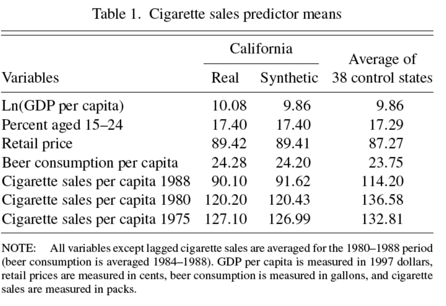
Abadie, Diamond, and Hainmueller (2010), Table 1.

For discussion: Compare California, synthetic California, and the donor-state average. Which predictors fit well, and where do differences remain?

California: Table 2

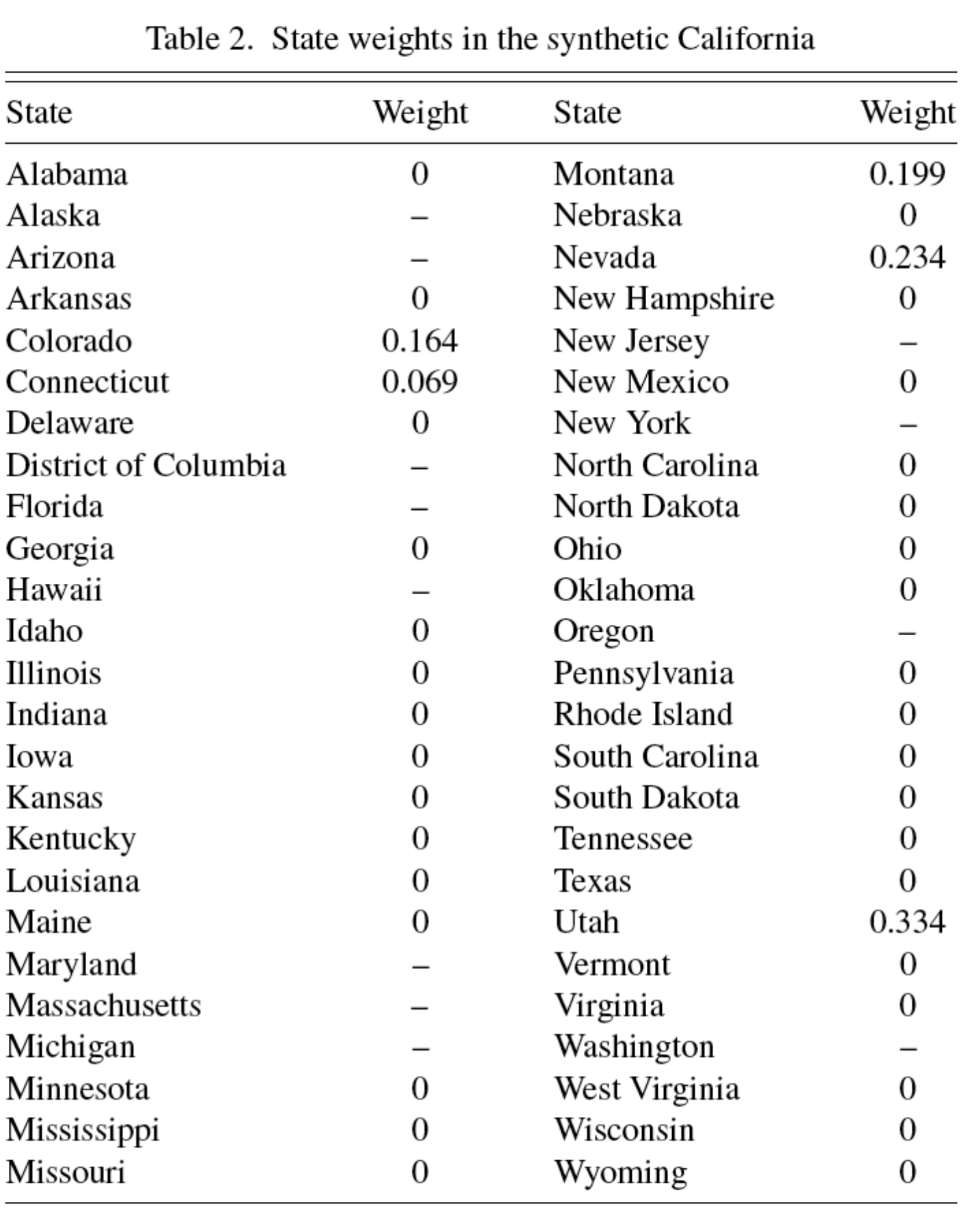
Abadie, Diamond, and Hainmueller (2010), Table 2.

For discussion: Which states contribute to synthetic California? Explain what a donor weight means and why many states receive zero weight.

California: Figure 3

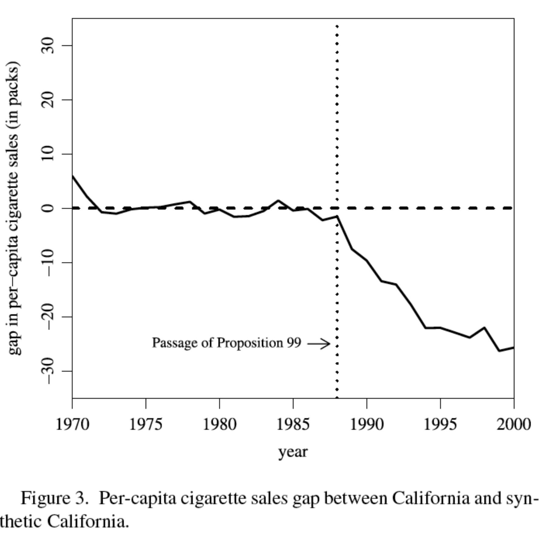
Abadie, Diamond, and Hainmueller (2010), Figure 3.

For discussion: Interpret the sign, units, and evolution of the gap. How convincing is the pre-treatment fit?

California: Figure 4

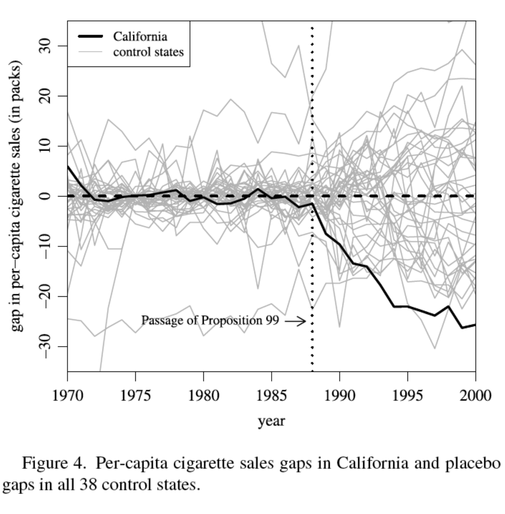
Abadie, Diamond, and Hainmueller (2010), Figure 4.

For discussion: How unusual is California relative to the placebo states? How does poor pre-treatment fit affect this comparison?

California: Figure 7

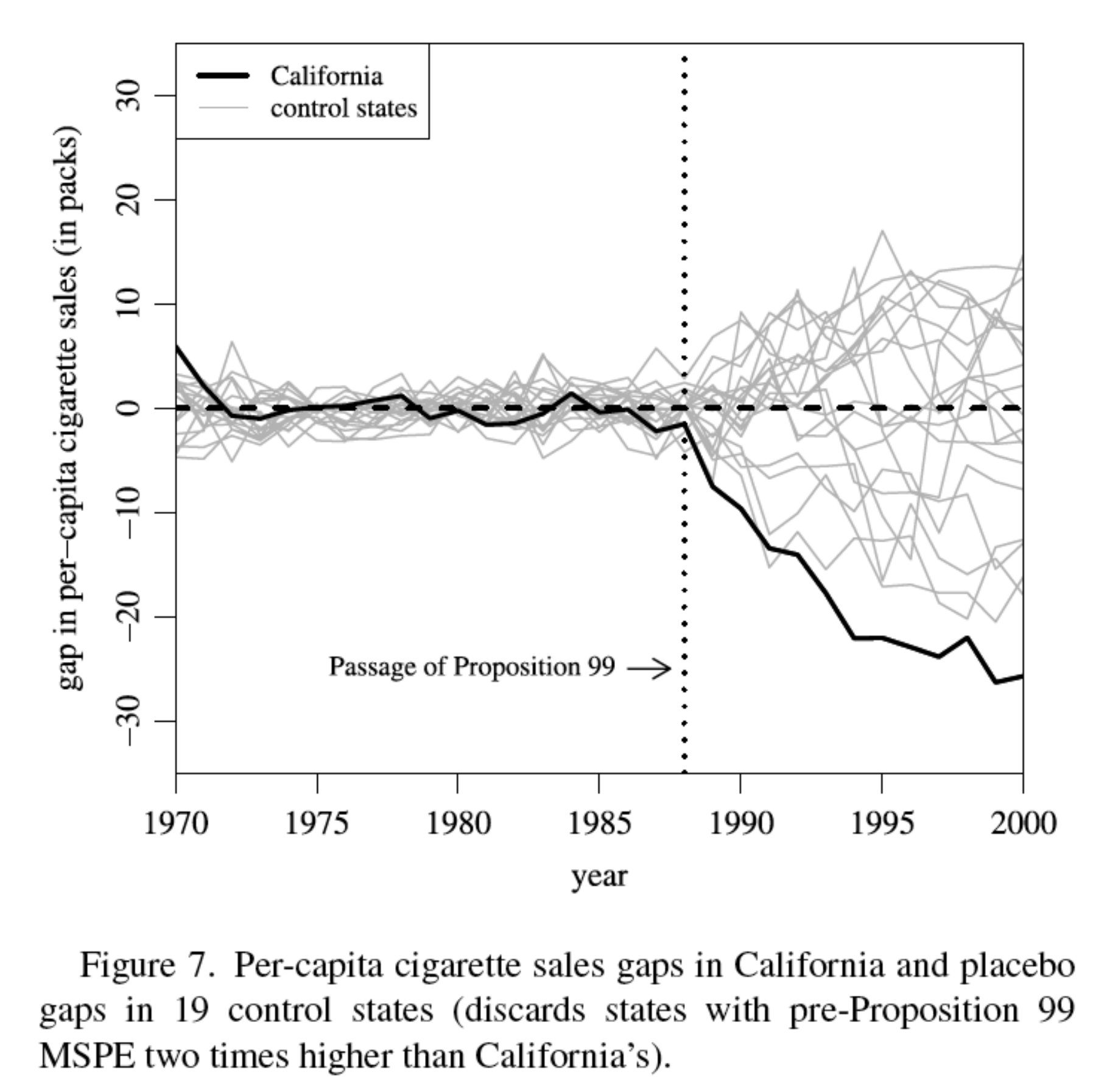
Abadie, Diamond, and Hainmueller (2010), Figure 7.

For discussion: How does the picture change when attention is restricted to placebos with better pre-treatment fit? What restriction did the authors use?

German Reunification: Policy and Data

For discussion: What is the outcome and which Germany is being studied? What is the intervention date?

Explain the proposed counterfactual and the choice of donor countries.

Could reunification also affect the donor countries?

The question concerns West German GDP per capita relative to a counterfactual without reunification. This is different from asking about GDP per capita for a newly combined East and West Germany. Spillovers through trade, finance, or European economic conditions matter for the donor comparison.

Reading the German Results: Erratum

The 2025 erratum corrects the GDP units to PPP current US dollars.

It also corrects the OECD sample averages in Table 2.

Use the corrected units when interpreting the figures and dollar gaps.

The original figure labels are retained in the reproduced exhibits. Read them with the corrected units. We use the erratum’s corrected predictor table below. See the erratum.

Germany: Figure 1

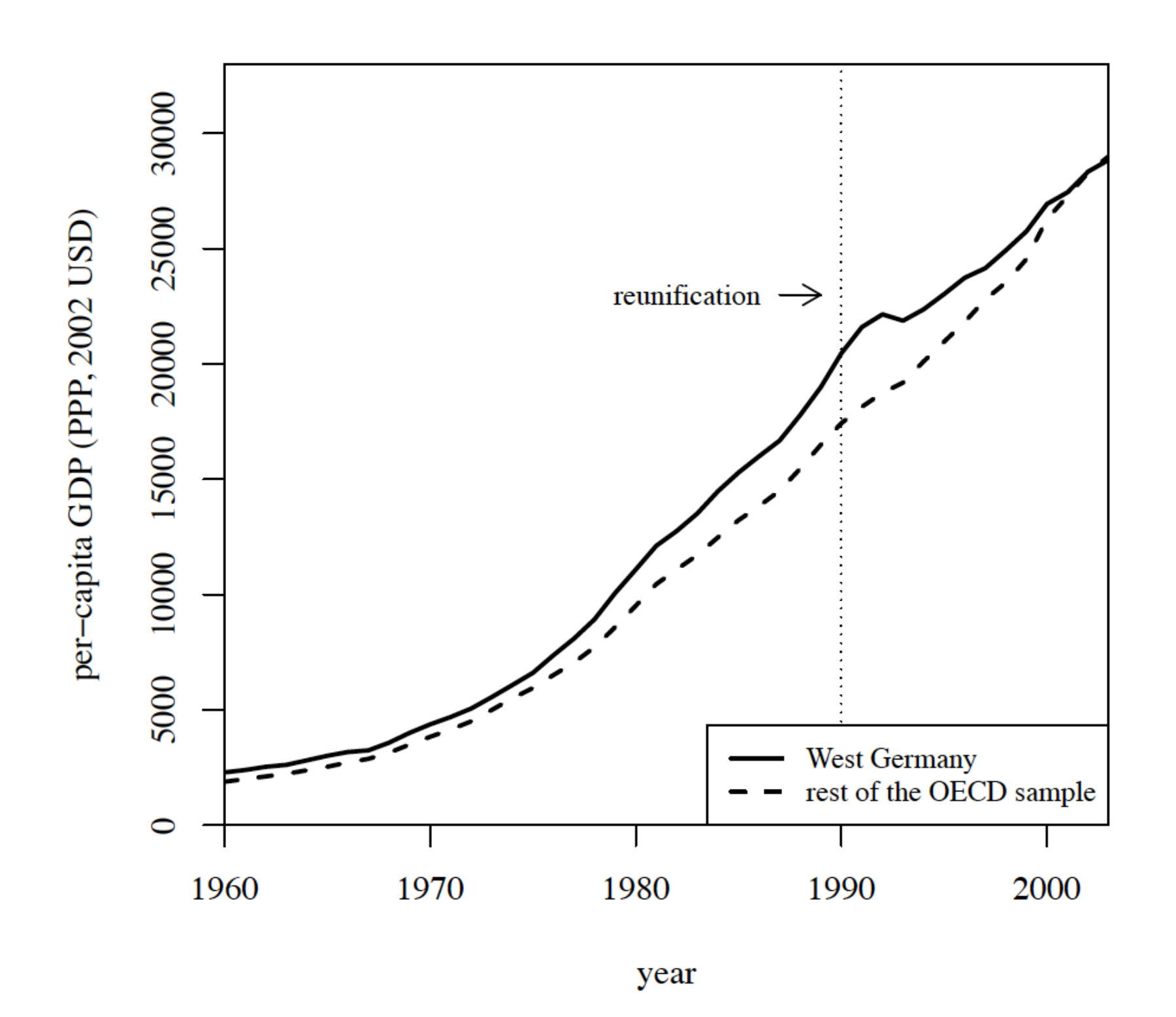
Abadie, Diamond, and Hainmueller (2015), Figure 1. GDP units: PPP current US dollars (2025 erratum).

For discussion: Does the OECD comparison follow West Germany before reunification? What should the synthetic control improve?

Where Do the Regression Weights Come From?

For each post-treatment year t, estimate across donor countries:

Y_{jt}=\beta_{0t}+\sum_{h=1}^{K}\beta_{ht}X_{hj}+u_{jt}.

Insert West Germany’s pre-treatment predictor values:

\widehat Y_{1t}^{0}=\widehat\beta_{0t} +\sum_{h=1}^{K}\widehat\beta_{ht}X_{h1}.

This prediction can be written as \sum_{j=2}^{J+1}w_j^{\mathrm{OLS}}Y_{jt}.

The table reports these implied country weights. They sum to one, but can be negative.

Each observation in the regression is a donor country. The dependent variable is its outcome in year t, and the explanatory variables are its pre-treatment predictors, including the selected summaries of past outcomes. The coefficients can differ across outcome years, hence the subscript t on each coefficient.

To predict West Germany’s untreated outcome, evaluate that fitted relationship at West Germany’s predictor values. OLS predictions can be expressed as weighted sums of the outcomes used to estimate the regression. Rewriting the prediction this way reveals each donor country’s contribution. These country weights are distinct from the regression coefficients on the predictors.

With the same predictors and donor sample across years, the implied country weights are the same in each year. Including an intercept makes them sum to one. Some weights can be negative or greater than one, allowing extrapolation beyond the donor countries.

Under the full-rank condition described by Abadie, these weights also reproduce the treated unit’s predictor values exactly. An exact predictor match can therefore be achieved through extrapolation. Inspecting the weights shows how the match is obtained. Synthetic control’s nonnegative weights keep the comparison within the available weighted averages and make any remaining predictor discrepancies visible. See Abadie (2021), Section 4, pp. 405–407.

Germany: Table 1

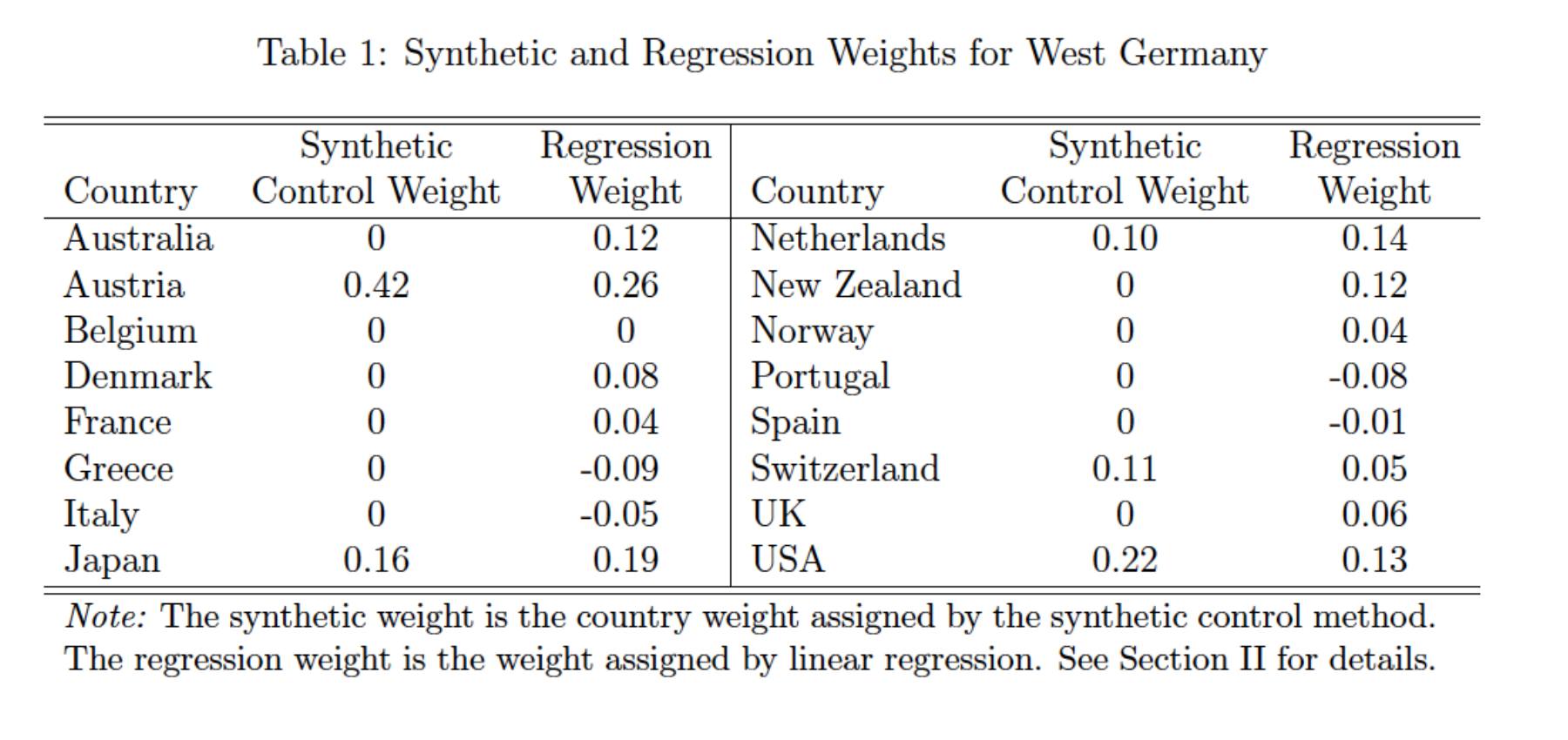
Abadie, Diamond, and Hainmueller (2015), Table 1.

For discussion: Compare the synthetic-control and regression weights. What does each method permit, and which countries drive the synthetic comparison?

Germany: Corrected Table 2

Predictor	West Germany	Synthetic West Germany	OECD sample
GDP per capita	15808.9	15802.2	15037.8
Trade openness	56.8	56.9	35.3
Inflation rate	2.6	3.5	5.7
Industry share	34.5	34.4	34.2
Schooling	55.5	55.2	44.4
Investment rate	27.0	27.0	25.7

Abadie, Diamond, and Hainmueller (2025), erratum, Table 1 correcting the 2015 Table 2. GDP: PPP current US dollars.

For discussion: How does synthetic West Germany compare with the OECD average as a match for West Germany?

GDP, openness, inflation, and industry share are averaged over 1981–1990. Schooling and investment use 1980–1985. The OECD column is weighted by 1990 population across the 16 donor countries. These are predictor means rather than treatment effects.

Germany: Figure 2

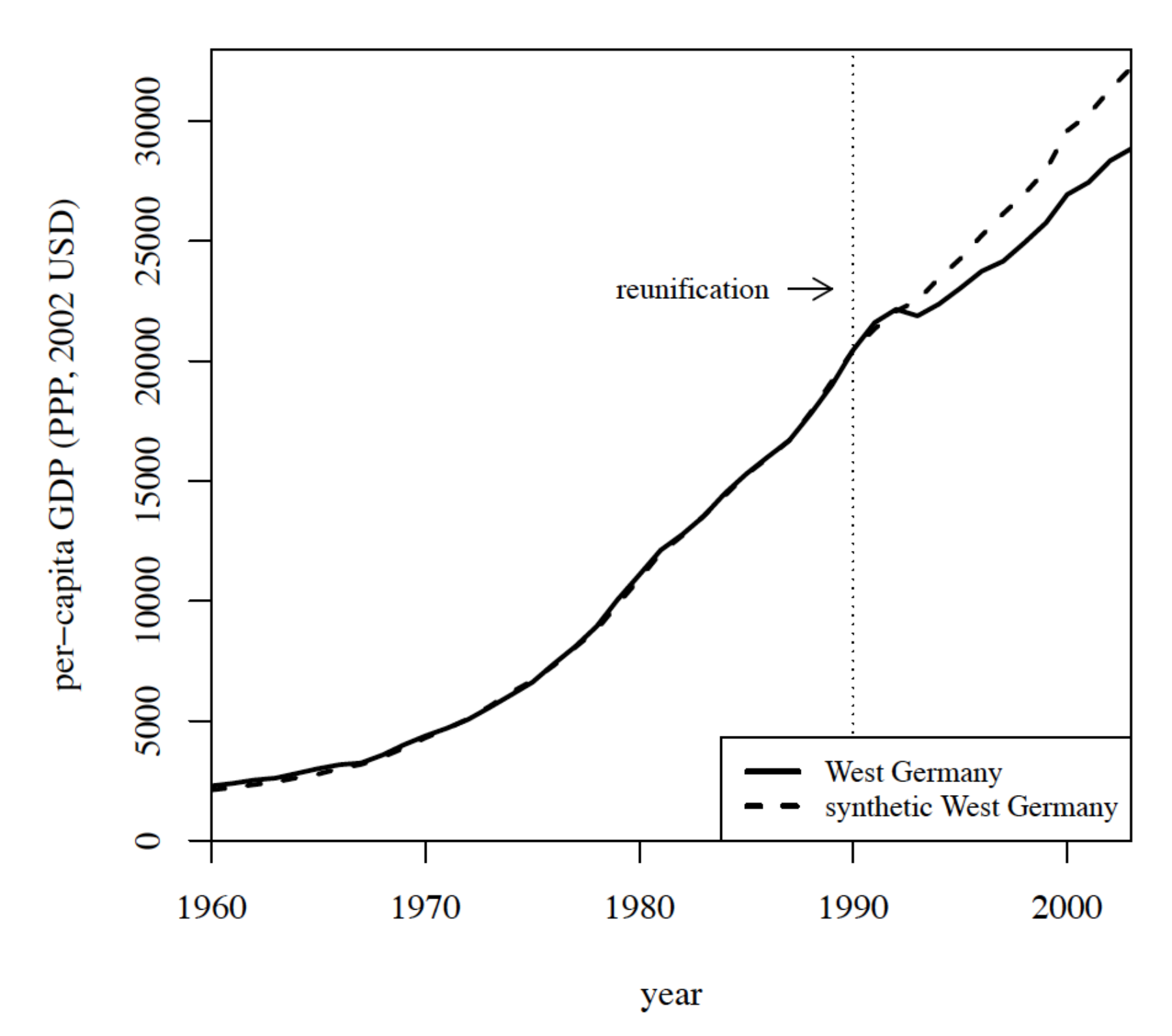
Abadie, Diamond, and Hainmueller (2015), Figure 2. GDP units: PPP current US dollars (2025 erratum).

For discussion: How closely does synthetic West Germany track the observed path before reunification? When do the paths diverge?

Germany: Figure 3

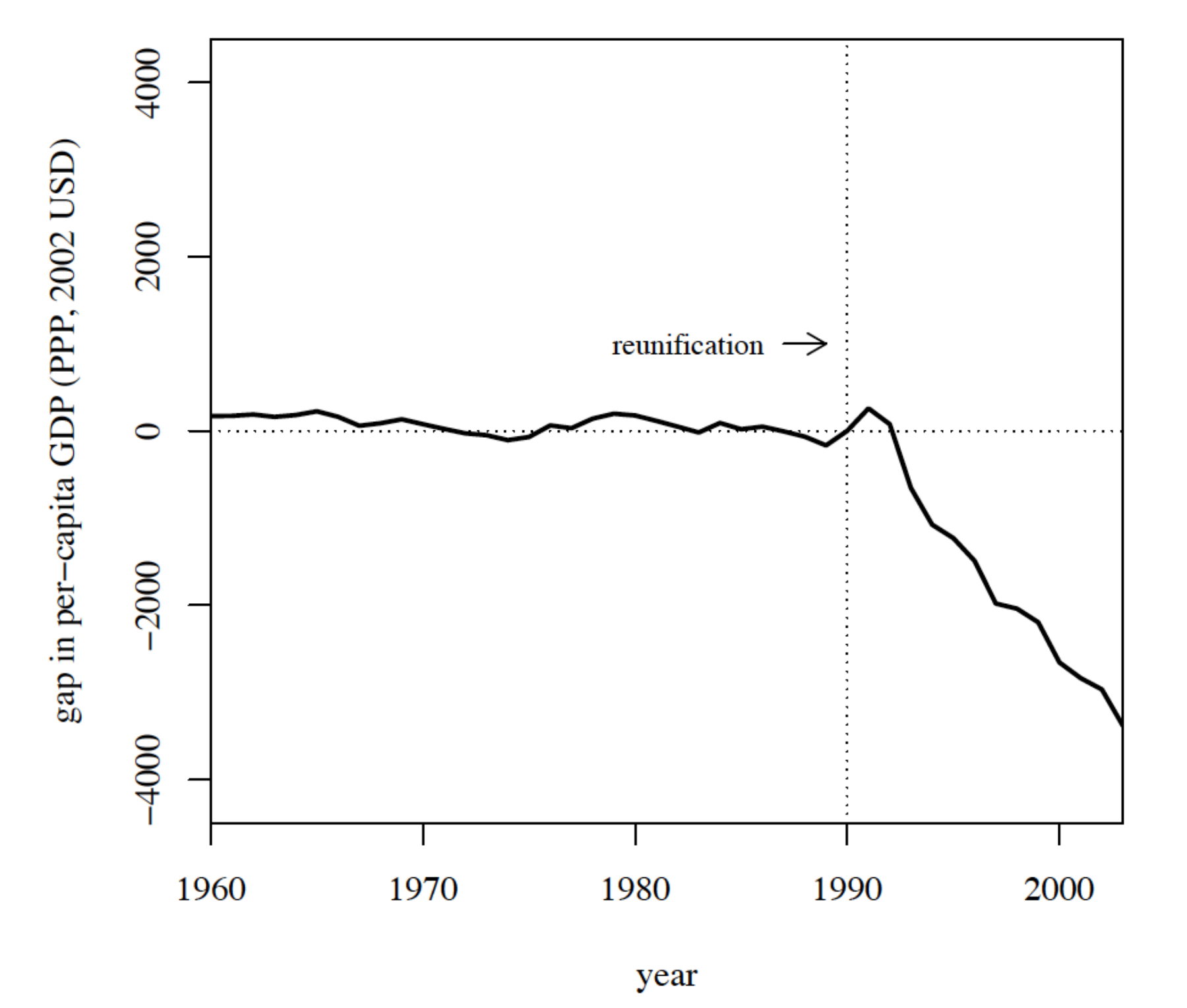
Abadie, Diamond, and Hainmueller (2015), Figure 3. GDP units: PPP current US dollars (2025 erratum).

For discussion: Interpret the size and evolution of the gap. What assumptions let us attribute this gap to reunification?

Germany: Figure 4

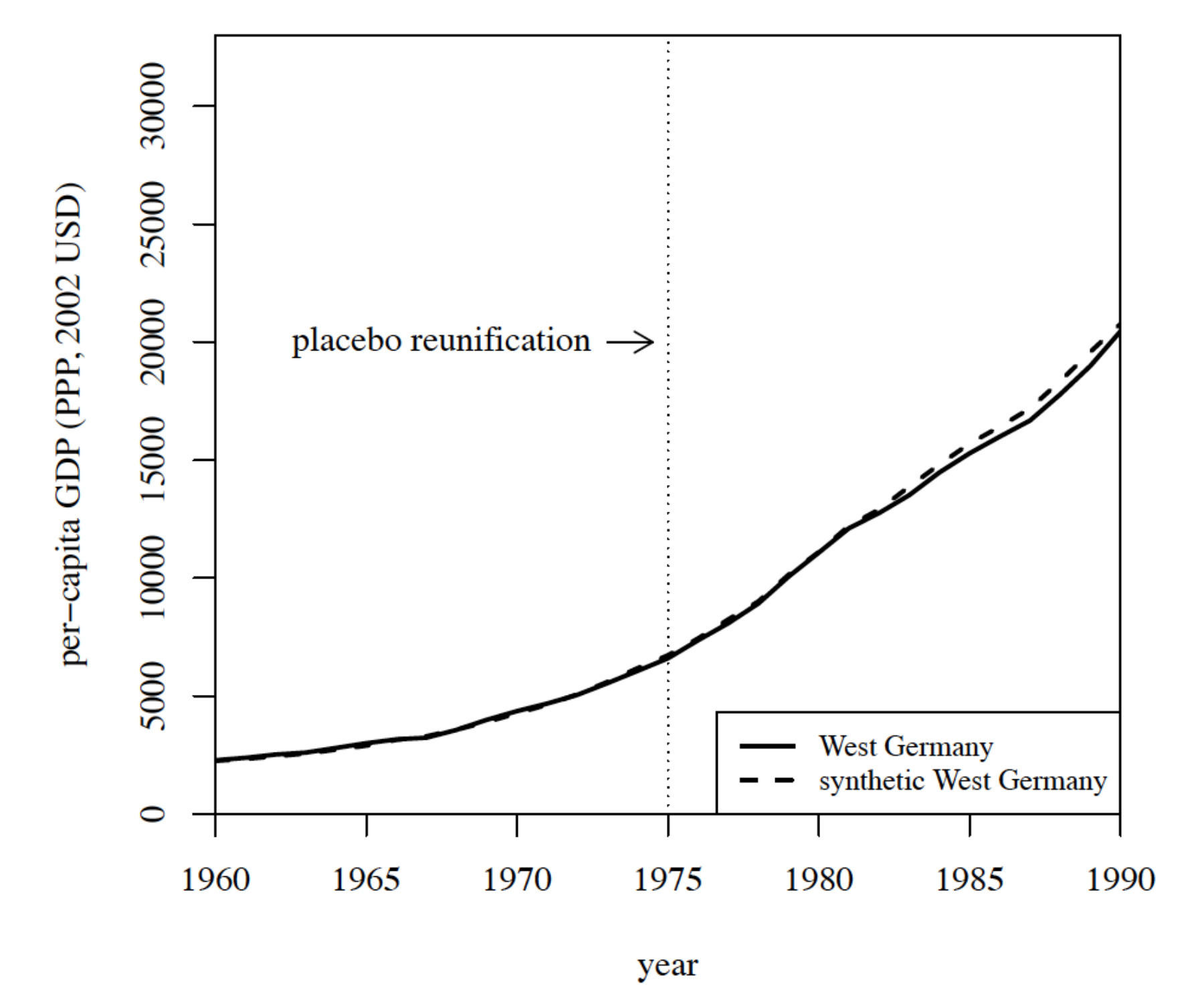
Abadie, Diamond, and Hainmueller (2015), Figure 4. GDP units: PPP current US dollars (2025 erratum).

For discussion: Why use a placebo reunification in 1975? Which observations should be used to fit that synthetic control?

Germany: Figure 6

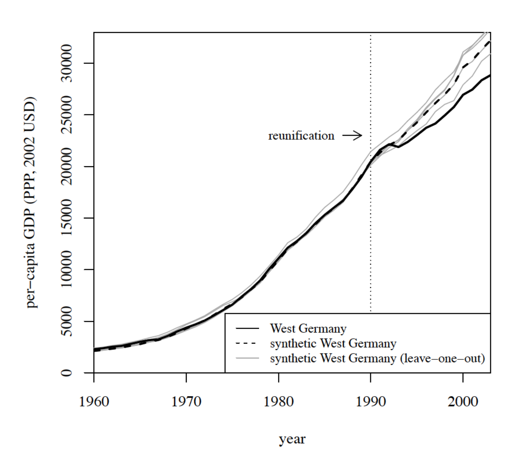
Abadie, Diamond, and Hainmueller (2015), Figure 6. GDP units: PPP current US dollars (2025 erratum).

For discussion: What is changed in each leave-one-out estimate? Does any single donor appear essential to the result?

Germany: Figure 7

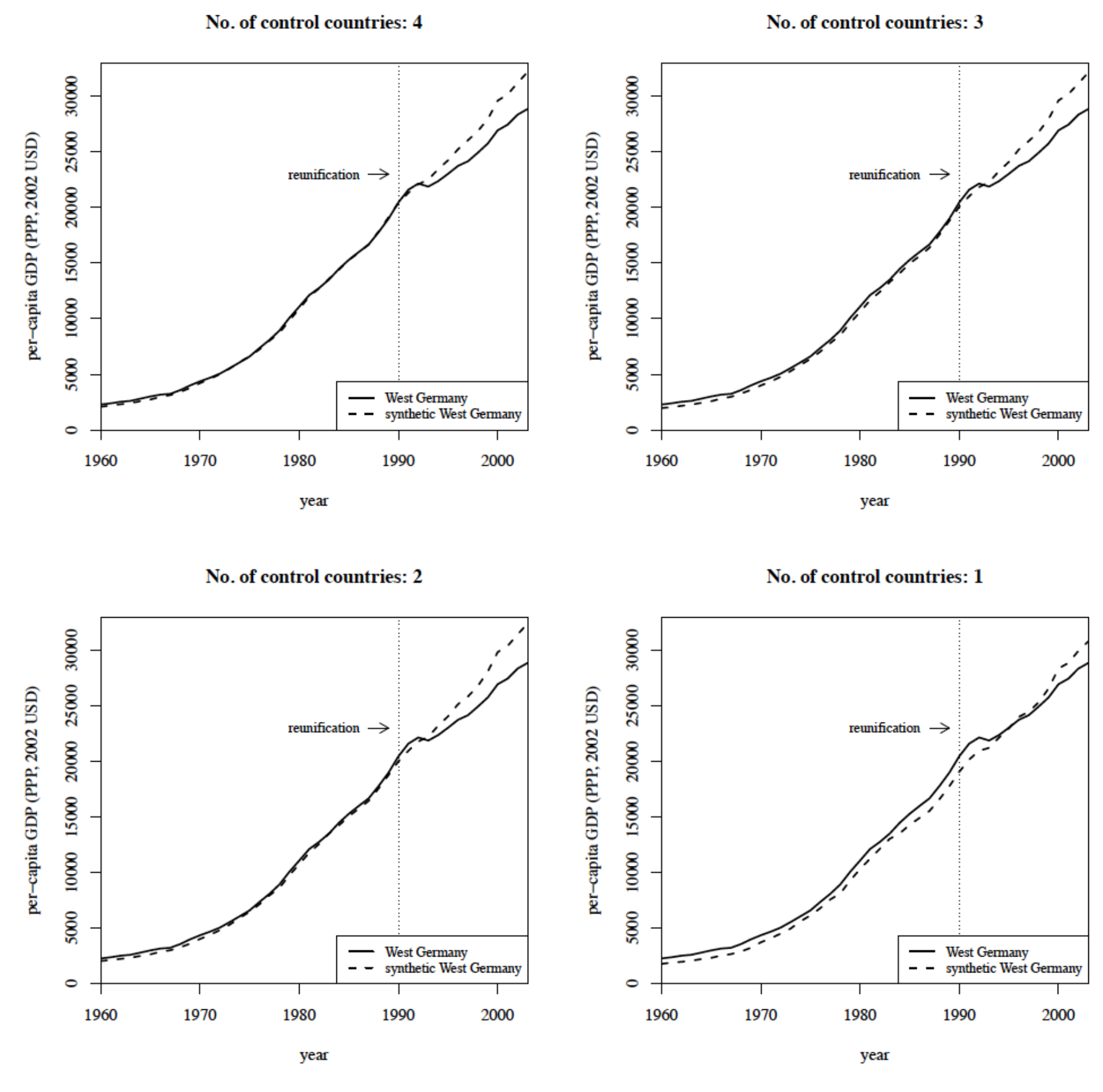
Abadie, Diamond, and Hainmueller (2015), Figure 7. GDP units: PPP current US dollars (2025 erratum).

For discussion: How do the conclusions change when fewer countries are used? Compare pre-treatment fit as well as the post-treatment paths.

Assessing the Two Applications

• Is the donor pool substantively credible?
• Does the synthetic control fit the pre-treatment outcomes?
• Could anticipation, spillovers, or other shocks explain the gap?
• Is the gap unusual relative to credible placebos?
• Does the conclusion survive reasonable changes in the comparison?

A donor receiving most of the weight is a reason to inspect sensitivity. It may be a particularly good comparison. The quality of the design depends on the credibility of that comparison and on the assumptions connecting its outcome to the treated unit’s missing untreated path.

Synthetic Control Requires Choices

Researchers choose the donor pool, predictors, pre-treatment window, validation period, and fitting procedure.

Report those choices and show the donor weights, fit, outcome paths, and sensitivity checks.

For policy, connect the estimated gap to the intervention and the population it represents.

An effect for one place and one historical intervention does not automatically describe the effect of adopting the policy elsewhere. Consider the mechanisms, economic conditions, and features of the policy that would need to carry over.

Post-Class Exercise

Construct synthetic West Germany using the supplied Python setup notebook. Compare donor weights and fit, plot the estimated effects, remove an influential donor, and examine placebo gaps. This is ungraded practice.

References

• Abadie, A., A. Diamond, and J. Hainmueller (2010). “Synthetic Control Methods for Comparative Case Studies: Estimating the Effect of California’s Tobacco Control Program.” JASA 105(490): 493–505. Link.
• Abadie, A., A. Diamond, and J. Hainmueller (2015). “Comparative Politics and the Synthetic Control Method.” AJPS 59(2): 495–510. Link. See also the 2025 erratum.
• Abadie, A. (2021). “Using Synthetic Controls: Feasibility, Data Requirements, and Methodological Aspects.” JEL 59(2): 391–425. Link.
• Kaul, A., S. Klössner, G. Pfeifer, and M. Schieler (2022). “Standard Synthetic Control Methods: The Case of Using All Preintervention Outcomes Together With Covariates.” JBES 40(3): 1362–1376.