---
title: "Week 3: Instrumental Variables and LATE"
subtitle: "The Oregon Health Insurance Experiment"
---
[Class slides](../slides/03-iv-late.qmd) · [Download slides as PDF](../resources/slides/03-iv-late.pdf) · [After-class exercise](../exercises/03-iv-late.qmd) · [Download notes as PDF](../resources/notes/03-iv-late.pdf) · [Download Quarto source](../resources/sessions/03-iv-late.qmd)
Prepare discussion items individually. The discussant list is provided separately on Moodle.
## Learning Objectives
By the end of this topic, you should be able to:
- Explain why omitted variables can bias OLS and how a valid instrument supplies variation that identifies a causal effect.
- Derive the Wald and exactly identified IV estimators using the analogy principle and moment conditions, and explain their connection to two-stage least squares.
- State the assumptions for LATE and explain the steps showing why the IV estimate identifies the effect for compliers.
- Distinguish the effects of winning the Oregon lottery and receiving Medicaid, and interpret what the estimates imply for policy.
## Before class {#readings}
Read these notes and Finkelstein et al. (2012), **“The Oregon Health Insurance Experiment: Evidence from the First Year.”** Focus on the lottery and data in Sections II–III, the empirical framework in Section IV, and **Tables II, III, IV, V, VIII, and IX**. [Published paper](https://doi.org/10.1093/qje/qjs020) · [Paper from Amy Finkelstein's website](https://economics.mit.edu/research/publications/oregon-health-insurance-experiment-evidence-first-year-0).
### Textbook references
- **The Effect:** [Chapter 19, Instrumental Variables](https://theeffectbook.net/ch-InstrumentalVariables.html), particularly the explanation of the IV comparison and local average treatment effects.
- **Causal Inference: The Remix:** [Chapter 7, Instrumental Variables](https://mixtape.scunning.com/07-instrumental_variables), particularly the Wald estimator, two-stage least squares, and LATE.
- **Mastering 'Metrics:** Chapter 3, *Instrumental Variables*. [Companion resources](https://www.masteringmetrics.com/online-metrics-resources/mastering-iv/) · [Mastering Econometrics videos at Marginal Revolution University](https://learn.mru.org/courses/mastering-econometrics).
- **Mostly Harmless Econometrics — optional advanced reading:** Chapter 4, especially Sections 4.1 and 4.4 on IV and heterogeneous effects. [Book contents](https://www.mostlyharmlesseconometrics.com/book-contents/).
Use these books for complementary explanations. **Additional reading:** Angrist and Krueger (2001), [“Instrumental Variables and the Search for Identification: From Supply and Demand to Natural Experiments”](https://doi.org/10.1257/jep.15.4.69), *Journal of Economic Perspectives* 15(4): 69–85.
## 1. From selection on observables to instrumental variables
Last week, we constructed comparisons between treated and untreated individuals with similar observed characteristics. The identifying assumption was that those characteristics account for selection into treatment that is related to potential outcomes.
Suppose important determinants remain unobserved. For example, health needs can influence both whether someone obtains health insurance and how much health care they use. Comparing insured and uninsured people may therefore combine the effect of insurance with differences that would have existed without insurance.
An **instrument**, $Z_i$, supplies a source of variation in treatment whose relationship with the outcome can be given a causal interpretation. In Oregon, a lottery offered some people the opportunity to apply for Medicaid. Winning increased the probability of obtaining insurance. It did not guarantee that a person enrolled.
We distinguish three variables:
| Symbol | Meaning in the Oregon application |
|:--|:--|
| $Z_i$ | Household selected by the lottery |
| $D_i$ | Individual obtains Medicaid coverage |
| $Y_i$ | An outcome, such as having an outpatient visit |
The effect of the **offer** and the effect of **receiving insurance** answer different policy questions. IV connects the two.
## 2. The Wald estimator
### Recall: omitted variables bias
The true population relationship is
$$Y_i=\beta_0+\beta_1D_i+\beta_2A_i+\nu_i,$$
where $Y_i$ is earnings, $D_i$ is **years of schooling**, and $A_i$ is ability. The coefficient $\beta_1$ is the causal effect of an additional year of schooling. We assume the remaining disturbance $\nu_i$ is uncorrelated with schooling and ability.
Recall the population regression of ability on schooling:
$$A_i=\gamma_0+\gamma_1D_i+v_i.$$
Substituting this relationship into the earnings equation gives
$$Y_i=\left(\beta_0+\beta_2\gamma_0\right)+\left(\beta_1+\beta_2\gamma_1\right)D_i+\beta_2v_i+\nu_i.$$
Thus the population slope of the short regression, which omits ability, is
$$\beta_1^{S}=\beta_1+\beta_2\gamma_1.$$
If ability raises earnings and is positively related to schooling, the short regression overstates the causal effect of schooling.
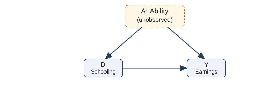
The backdoor path $D\leftarrow A\rightarrow Y$ connects schooling and earnings through ability. The short regression combines the causal effect along $D\rightarrow Y$ with this additional association.
### Bias and unbiasedness of OLS
The estimated slope changes from sample to sample. Its **sampling distribution** describes the values we would obtain by repeatedly drawing samples of the same size from the same population. The **bias** of the estimator, relative to the causal effect $\beta_1$, is
$$\operatorname{Bias}\left(\widehat\beta_1^{S}\right)=E\left[\widehat\beta_1^{S}\right]-\beta_1.$$
Here the expectation is over repeated samples. An estimator is **unbiased** if its mean across those samples equals the parameter it estimates. Individual estimates can still be above or below that parameter.
To derive the expectation of the OLS slope, imagine repeatedly observing outcomes for the same schooling values. Write the collection of schooling values as $\mathbf D=\left(D_1,\ldots,D_n\right)$, and suppose there is variation in schooling. Starting with $Y_i=\beta_0+\beta_1D_i+u_i$, the sample OLS formula gives
$$\begin{aligned}
\widehat\beta_1^{S}
&=\frac{\sum_i\left(D_i-\overline D\right)Y_i}{\sum_i\left(D_i-\overline D\right)^2}\\
&=\beta_1+\frac{\sum_i\left(D_i-\overline D\right)u_i}{\sum_i\left(D_i-\overline D\right)^2}.
\end{aligned}$$
The intercept drops out because $\sum_i\left(D_i-\overline D\right)=0$. Conditional on $\mathbf D$, both the denominator and each $D_i-\overline D$ are fixed, so we can move them outside the expectation:
$$E\left[\widehat\beta_1^{S}\mid\mathbf D\right]=\beta_1+
\frac{\sum_i\left(D_i-\overline D\right)E\left[u_i\mid\mathbf D\right]}{\sum_i\left(D_i-\overline D\right)^2}.$$
Under the **zero conditional mean assumption**, $E\left[u_i\mid\mathbf D\right]=0$, the second term is zero. The estimator is therefore unbiased conditional on the schooling values. Averaging over possible sets of schooling values also gives $E\left[\widehat\beta_1^{S}\right]=\beta_1$, provided the expectation exists. Conditioning allows us to do the calculation even when schooling is random in the population.
When ability is omitted, $u_i=\beta_2A_i+\nu_i$. If ability is related to schooling, the zero conditional mean assumption generally fails. The fraction in the conditional-expectation expression shows how the resulting conditional bias arises. The earlier expression $\beta_1^{S}=\beta_1+\beta_2\gamma_1$ describes the population short-regression slope; here we have examined the expectation of its sample estimator relative to the causal effect.
### From the conditional expectation to the covariance formula
Substitute $u_i=\beta_2A_i+\nu_i$ into the conditional expectation above and assume $E\left[\nu_i\mid\mathbf D\right]=0$:
$$E\left[\widehat\beta_1^{S}\mid\mathbf D\right]=\beta_1+\beta_2
\frac{\sum_i\left(D_i-\overline D\right)E\left[A_i\mid\mathbf D\right]}{\sum_i\left(D_i-\overline D\right)^2}.$$
The fraction is the conditional expectation of the sample slope from regressing ability on schooling, $E\left[\widehat\gamma_1\mid\mathbf D\right]$. This follows by applying the same OLS formula to that auxiliary regression:
$$\widehat\gamma_1=\frac{\sum_i\left(D_i-\overline D\right)A_i}{\sum_i\left(D_i-\overline D\right)^2}.$$
To obtain the familiar population covariance expression for the finite-sample bias, now assume the **conditional mean of ability is linear in schooling**:
$$E\left[A_i\mid\mathbf D\right]=\gamma_0+\gamma_1D_i.$$
Equivalently, the residual in $A_i=\gamma_0+\gamma_1D_i+v_i$ has conditional mean zero given the schooling values. This is an additional assumption beyond merely writing the population regression.
The numerator simplifies to
$$\begin{aligned}
\sum_i\left(D_i-\overline D\right)E\left[A_i\mid\mathbf D\right]
&=\sum_i\left(D_i-\overline D\right)\left(\gamma_0+\gamma_1D_i\right)\\
&=\gamma_1\sum_i\left(D_i-\overline D\right)^2.
\end{aligned}$$
The intercept term vanishes because the deviations from the sample mean sum to zero. The remaining sum cancels the denominator, giving
$$E\left[\widehat\beta_1^{S}\mid\mathbf D\right]=\beta_1+\beta_2\gamma_1.$$
The population slope in the ability-on-schooling regression is $\gamma_1=\operatorname{Cov}\left(A_i,D_i\right)/\operatorname{Var}\left(D_i\right)$. Therefore,
$$E\left[\widehat\beta_1^{S}\mid\mathbf D\right]
=\beta_1+\beta_2\frac{\operatorname{Cov}\left(A_i,D_i\right)}{\operatorname{Var}\left(D_i\right)}.$$
Under these assumptions, the conditional bias relative to the causal effect is $\beta_2\gamma_1$. Averaging over schooling samples yields the same unconditional bias, provided the expectation exists. If ability raises earnings and is positively related to schooling, this bias is positive.
**What can we do if ability is unobserved?**
### A binary instrument
Write the earnings equation as $Y_i=\beta_0+\beta_1D_i+u_i$, with $u_i=\beta_2A_i+\nu_i$.
Suppose we have a binary instrument, $Z_i$, that has **two properties at the same time**:
$$E\left[u_i\mid Z_i=1\right]=E\left[u_i\mid Z_i=0\right]=0,$$
$$E\left[D_i\mid Z_i=1\right]\ne E\left[D_i\mid Z_i=0\right].$$
The instrument shifts schooling and affects earnings through schooling. We call the first relationship the **orthogonality assumption** and the second relationship the **relevance assumption**.
Finding a variable with either property is easy. The challenge is finding one that satisfies **both at the same time**: it predicts years of schooling while remaining uncorrelated with the unobserved determinants of earnings. For example, an independently generated random number can satisfy orthogonality, but will not predict schooling in the population. Ability predicts schooling, but is part of the unobserved determinants of earnings.
The **exclusion restriction** requires the instrument to affect earnings through schooling. Together with independence from the other determinants of earnings, it supports the orthogonality condition above, where we have normalised the mean of $u_i$ to zero.
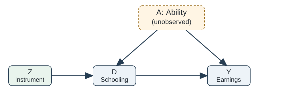
The arrow $Z\rightarrow D$ represents relevance. Exclusion requires the effect of $Z$ on earnings to operate through schooling, and independence requires $Z$ to be independent of ability and the other unobserved determinants of earnings. Together, exclusion and independence support the orthogonality assumption.
Taking conditional expectations:
$$\begin{aligned}
E\left[Y_i\mid Z_i=1\right]&=\beta_0+\beta_1E\left[D_i\mid Z_i=1\right],\\
E\left[Y_i\mid Z_i=0\right]&=\beta_0+\beta_1E\left[D_i\mid Z_i=0\right].
\end{aligned}$$
Subtract the second equation from the first:
$$E\left[Y_i\mid Z_i=1\right]-E\left[Y_i\mid Z_i=0\right]
=\beta_1\left[E\left[D_i\mid Z_i=1\right]-E\left[D_i\mid Z_i=0\right]\right].$$
Solving for the causal effect gives
$$\beta_1=\frac{E\left[Y_i\mid Z_i=1\right]-E\left[Y_i\mid Z_i=0\right]}{E\left[D_i\mid Z_i=1\right]-E\left[D_i\mid Z_i=0\right]}.$$
Using the **analogy principle** to replace the population conditional means with the sample conditional means gives the **Wald estimator**:
$$\widehat\beta_{1,\mathrm{Wald}}=\frac{\overline{Y}_{Z=1}-\overline{Y}_{Z=0}}{\overline{D}_{Z=1}-\overline{D}_{Z=0}}.$$
The instrument-induced difference in outcomes equals the causal effect multiplied by the instrument-induced difference in treatment. Dividing by the treatment difference recovers the effect per unit of treatment.
### An illustrative schooling and earnings model
For this illustration, the simulated relationships are
$$D_i=11+5Z_i+1.8A_i+v_i,\qquad Y_i=100+5D_i+20A_i+\nu_i,$$
where $Z_i$ is Bernoulli with probability one-half, and $A_i$, $v_i$, and $\nu_i$ are mutually independent, mean-zero normal variables, independent of $Z_i$. Their standard deviations are 1, 0.65, and 10 respectively. The figure uses 400 observations. These are simulated data used to illustrate the geometry.
The true effect of an additional year of schooling is 5. Independence of the variables used to generate schooling gives
$$\operatorname{Cov}\left(A_i,D_i\right)=1.8\operatorname{Var}\left(A_i\right)=1.8,$$
$$\operatorname{Var}\left(D_i\right)=25\operatorname{Var}\left(Z_i\right)+1.8^2\operatorname{Var}\left(A_i\right)+\operatorname{Var}\left(v_i\right)=6.25+3.24+0.4225=9.9125.$$
Thus the population slope of earnings on schooling when ability is omitted is
$$\beta_1^S=5+20\frac{1.8}{9.9125}\approx8.63.$$
The population omitted-variable bias is approximately 3.63. The sample OLS slope will vary around the population regression target; the covariance calculation here identifies that target without asserting exact finite-sample unbiasedness for this simulation.
### The graphical argument
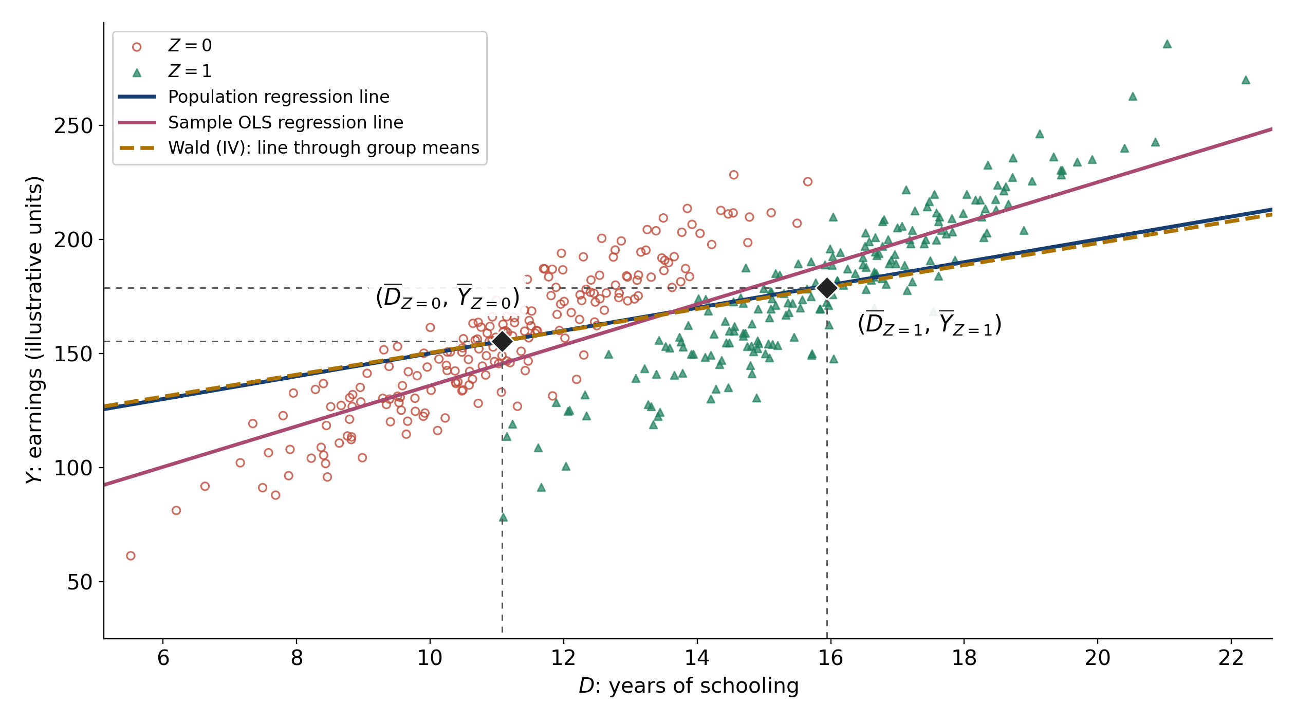
The **population regression line** has the true causal slope, $\beta_1=5$. Here ability raises both years of schooling and earnings, so the **sample OLS line** is too steep. The **Wald (IV) line** passes through the two sample mean points, $\left(\overline{D}_{Z=0},\overline{Y}_{Z=0}\right)$ and $\left(\overline{D}_{Z=1},\overline{Y}_{Z=1}\right)$. Its slope is their vertical separation divided by their horizontal separation. The instrument shifts treatment independently of ability, allowing this comparison to recover the causal slope as the sample grows. In a finite sample, the IV and population lines can differ.
### Reproducing the figure in Python
First generate 400 observations from the relationships above. Setting a random seed gives us the same data each time we run the code. Ability enters both equations, while the instrument is generated independently of ability and the disturbances.
```{python}
#| label: wald-simulate
import numpy as np
import pandas as pd
import statsmodels.formula.api as smf
import matplotlib.pyplot as plt

rng = np.random.default_rng(20260923)
n = 400

Z = rng.binomial(n=1, p=0.5, size=n)
A = rng.normal(loc=0, scale=1, size=n)
nu = rng.normal(loc=0, scale=10, size=n)
v = rng.normal(loc=0, scale=0.65, size=n)

D = 11 + 5 * Z + 1.8 * A + v
Y = 100 + 5 * D + 20 * A + nu

simulated = pd.DataFrame({"Y": Y, "D": D, "Z": Z, "A": A})
simulated.head()
```
Next estimate OLS and calculate the Wald estimator from the two instrument-group means. The intercept of the IV line is chosen so that it passes through the mean point for $Z=0$; the Wald slope ensures it also passes through the mean point for $Z=1$.
```{python}
#| label: wald-estimate
ols = smf.ols("Y ~ D", data=simulated).fit(cov_type="HC1")
means = simulated.groupby("Z")[["D", "Y"]].mean()

wald_slope = (
    (means.loc[1, "Y"] - means.loc[0, "Y"])
    / (means.loc[1, "D"] - means.loc[0, "D"])
)
wald_intercept = means.loc[0, "Y"] - wald_slope * means.loc[0, "D"]

pd.DataFrame({
    "Line": ["Population", "Sample OLS", "Wald (IV)"],
    "Slope": [5, ols.params["D"], wald_slope]
}).round(3)
```
Finally, plot the observations, the three lines, and the group means. The dashed horizontal and vertical guides locate each mean point on the axes.
```{python}
#| label: fig-wald-simulation
#| fig-show: hide
#| fig-cap: "The Wald line connects the two instrument-group means. Simulated data."
#| fig-width: 12
#| fig-height: 6.7
#| fig-alt: "Open circles indicate Z=0 and triangles Z=1. The sample OLS line is steeper than the population line; the Wald line passes through the two group means and is close to the population line."
plt.rcParams.update({"font.size": 14, "font.family": "DejaVu Sans"})
fig, ax = plt.subplots(figsize=(12, 6.7))

group0 = simulated.loc[simulated["Z"] == 0]
group1 = simulated.loc[simulated["Z"] == 1]
ax.scatter(group0["D"], group0["Y"], s=27, marker="o",
           facecolors="none", edgecolors="#c04b38", alpha=0.8,
           linewidths=1.1, label="$Z=0$")
ax.scatter(group1["D"], group1["Y"], s=25, marker="^",
           color="#20815d", alpha=0.7, label="$Z=1$")

# Evaluate each line over the range of observed treatment values.
d_grid = np.linspace(simulated["D"].min() - 0.4,
                     simulated["D"].max() + 0.4, 250)
ax.plot(d_grid, 100 + 5 * d_grid, color="#163e70", linewidth=2.6,
        label="Population regression line")
ax.plot(d_grid, ols.params["Intercept"] + ols.params["D"] * d_grid,
        color="#ab4a71", linewidth=2.4, label="Sample OLS regression line")
ax.plot(d_grid, wald_intercept + wald_slope * d_grid,
        color="#ac7300", linewidth=2.6, linestyle="--",
        label="Wald (IV): line through group means")

ax.set_xlim(d_grid[0], d_grid[-1])
ax.set_ylim(25, 295)
for z in [0, 1]:
    mean_d = means.loc[z, "D"]
    mean_y = means.loc[z, "Y"]
    ax.plot([d_grid[0], mean_d, mean_d], [mean_y, mean_y, 25],
            color="#555555", linestyle=(0, (4, 4)), linewidth=1)
    ax.scatter(mean_d, mean_y, s=120, marker="D", color="#222222",
               edgecolors="white", zorder=8)
    label = (r"$(\overline{D}_{Z=" + str(z)
             + r"},\,\overline{Y}_{Z=" + str(z) + r"})$")
    offset = (-85, 24) if z == 0 else (20, -30)
    ax.annotate(label, (mean_d, mean_y), xytext=offset,
                textcoords="offset points", fontsize=15, zorder=9,
                bbox={"facecolor": "white", "edgecolor": "none", "alpha": 0.9})

ax.set_xlabel("$D$: years of schooling")
ax.set_ylabel("$Y$: earnings (illustrative units)")
ax.spines[["top", "right"]].set_visible(False)
ax.legend(loc="upper left", fontsize=11.5, framealpha=0.95)
fig.tight_layout()
plt.close(fig)
```
## 3. From Wald to instrumental variables
### First stage and reduced form
The **first stage** regresses the endogenous explanatory variable on **all the exogenous variables**. The **reduced form** regresses the outcome on **all the exogenous variables**. Both include the excluded instrument(s), any included exogenous covariates, and an intercept.
The terminology comes from **simultaneous-equations models**. We solve the system to express each endogenous variable as a function of all the exogenous variables and a disturbance. In IV applications, “the reduced form” usually refers to the equation for the outcome $Y_i$. The first-stage equation for $D_i$ is also a reduced-form equation.
In our simplest example, substitute the first-stage relationship $D_i=\pi_0+\pi_1Z_i+v_i$ into the earnings equation $Y_i=\beta_0+\beta_1D_i+u_i$:
$$\begin{aligned}
Y_i&=\beta_0+\beta_1\left(\pi_0+\pi_1Z_i+v_i\right)+u_i\\
&=\left(\beta_0+\beta_1\pi_0\right)+\beta_1\pi_1Z_i+\left(u_i+\beta_1v_i\right)\\
&=\delta_0+\delta_1Z_i+e_i.
\end{aligned}$$
Thus $\delta_0=\beta_0+\beta_1\pi_0$, $\delta_1=\beta_1\pi_1$, and $e_i=u_i+\beta_1v_i$. The reduced-form coefficient on the instrument is the causal effect multiplied by the first-stage coefficient. Relevance permits us to divide by $\pi_1$, recovering $\beta_1=\delta_1/\pi_1$. When the model includes exogenous covariates, those covariates enter both the first stage and the reduced form as well.
Write the population regressions as
$$\begin{aligned}
D_i&=\pi_0+\pi_1Z_i+v_i &&\text{(first stage)},\\
Y_i&=\delta_0+\delta_1Z_i+e_i &&\text{(reduced form)}.
\end{aligned}$$
With one endogenous explanatory variable and one excluded instrument, the model is **exactly identified**. The IV estimate equals the reduced-form coefficient on that instrument divided by its first-stage coefficient, using the same sample, weights, and included exogenous covariates. This single-coefficient ratio applies to the one-instrument, one-endogenous-variable case.
With a binary instrument, each slope is the difference between the corresponding group means. Therefore Wald is the estimated reduced-form slope divided by the estimated first-stage slope: $\widehat\beta_{1,\mathrm{Wald}}=\widehat\delta_1/\widehat\pi_1$.
For $P\left(Z_i=1\right)=p$,
$$\operatorname{Cov}\left(Y_i,Z_i\right)=\left[E\left[Y_i\mid Z_i=1\right]-E\left[Y_i\mid Z_i=0\right]\right]p\left(1-p\right),$$
$$\operatorname{Cov}\left(D_i,Z_i\right)=\left[E\left[D_i\mid Z_i=1\right]-E\left[D_i\mid Z_i=0\right]\right]p\left(1-p\right).$$
The common factor cancels in their ratio:
$$\beta_1=\frac{\operatorname{Cov}\left(Y_i,Z_i\right)}{\operatorname{Cov}\left(D_i,Z_i\right)}
=\frac{\operatorname{Cov}\left(Y_i,Z_i\right)/\operatorname{Var}\left(Z_i\right)}{\operatorname{Cov}\left(D_i,Z_i\right)/\operatorname{Var}\left(Z_i\right)}.$$
This expresses IV as the reduced-form coefficient divided by the first-stage coefficient. The covariance ratio also applies to a continuous instrument when $\operatorname{Cov}\left(Z_i,u_i\right)=0$ and $\operatorname{Cov}\left(Z_i,D_i\right)\ne0$. Replacing these population covariances with sample covariances gives the IV estimator.
### IV as a method-of-moments estimator
The Wald estimator used the analogy principle: replace population conditional means with sample conditional means. We can construct IV in the same way from a population moment condition. This gives an estimator for either a binary or a continuous instrument.
Orthogonality concerns the covariance between the instrument and the **outcome disturbance**:
$$\begin{aligned}
0&=\operatorname{Cov}\left(Z_i,u_i\right)\\
&=E\left[\left(Z_i-E\left[Z_i\right]\right)\left(u_i-E\left[u_i\right]\right)\right]\\
&=E\left[\left(Z_i-E\left[Z_i\right]\right)u_i\right].
\end{aligned}$$
The “useful result” lets us drop the mean from the second term because $E\left[Z_i-E\left[Z_i\right]\right]=0$.
Now substitute $u_i=Y_i-\beta_0-\beta_1D_i$:
$$E\left[\left(Z_i-E\left[Z_i\right]\right)
\left(Y_i-\beta_0-\beta_1D_i\right)\right]=0.$$
To see the cancellation explicitly, the term removed is
$$E\left[\left(Z_i-E\left[Z_i\right]\right)E\left[u_i\right]\right]
=E\left[u_i\right]E\left[Z_i-E\left[Z_i\right]\right]=0.$$
Thus this simplification holds even without imposing $E\left[u_i\right]=0$. It is the familiar useful result: centring one variable is sufficient when calculating a covariance. We retain $u_i$ for the outcome disturbance and $v_i$ for the first-stage residual.
Apply the **analogy principle**, replacing the population mean of $Z_i$ with $\overline Z$ and the expectation with a sample average. Choose the estimated coefficients to satisfy
$$\frac{1}{n}\sum_i\left(Z_i-\overline Z\right)
\left(Y_i-\widehat\beta_0-\widehat\beta_1D_i\right)=0.$$
Multiply by $n$ and expand:
$$\sum_i\left(Z_i-\overline Z\right)Y_i
-\widehat\beta_0\sum_i\left(Z_i-\overline Z\right)
-\widehat\beta_1\sum_i\left(Z_i-\overline Z\right)D_i=0.$$
Because the centred instrument sums to zero, the intercept term vanishes. Rearranging gives
$$\widehat\beta_{1,\mathrm{IV}}=
\frac{\sum_i\left(Z_i-\overline Z\right)Y_i}
{\sum_i\left(Z_i-\overline Z\right)D_i}.$$
We can subtract $\overline Y$ in the numerator and $\overline D$ in the denominator without changing either sum, again because $\sum_i\left(Z_i-\overline Z\right)=0$. Thus
$$\widehat\beta_{1,\mathrm{IV}}=
\frac{\sum_i\left(Z_i-\overline Z\right)\left(Y_i-\overline Y\right)}
{\sum_i\left(Z_i-\overline Z\right)\left(D_i-\overline D\right)}
=\frac{\widehat{\operatorname{Cov}}\left(Z_i,Y_i\right)}
{\widehat{\operatorname{Cov}}\left(Z_i,D_i\right)}.$$
The common sample-covariance divisor cancels. This expression requires a nonzero sample covariance between the instrument and schooling; the identifying relevance condition requires the corresponding population covariance to be nonzero.
To estimate the intercept as well, use the population condition $E\left[u_i\right]=0$. Its sample counterpart is
$$\frac{1}{n}\sum_i\left(Y_i-\widehat\beta_0-\widehat\beta_{1,\mathrm{IV}}D_i\right)=0,$$
which gives $\widehat\beta_{0,\mathrm{IV}}=\overline Y-\widehat\beta_{1,\mathrm{IV}}\overline D$.
This is the **method of moments**: choose the coefficients so that the sample counterparts of the population moment conditions hold. For a binary instrument, the covariance ratio simplifies to the Wald ratio of differences in group means. Two-stage least squares provides another way to compute the same estimate.
### Using the instrument to predict treatment
Our goal is to isolate variation in treatment that is uncorrelated with the unobserved determinants of the outcome. The population first-stage regression gives the predicted component
$$D_i^*=\pi_0+\pi_1Z_i,\qquad \pi_1=\frac{\operatorname{Cov}\left(D_i,Z_i\right)}{\operatorname{Var}\left(Z_i\right)}.$$
Since this component is a linear function of the instrument,
$$\operatorname{Cov}\left(D_i^*,u_i\right)=\pi_1\operatorname{Cov}\left(Z_i,u_i\right)=0.$$
The first-stage residual is uncorrelated with $Z_i$ and hence with $D_i^*$. Writing $D_i=D_i^*+v_i$ in the outcome equation gives
$$Y_i=\beta_0+\beta_1D_i^*+\left(\beta_1v_i+u_i\right).$$
Thus $D_i^*$ is uncorrelated with the disturbance in this equation. In a sample, we estimate this predicted component with $\widehat D_i=\widehat\pi_0+\widehat\pi_1Z_i$. This leads directly to two-stage least squares.
### Dividing schooling into exogenous and endogenous components
The fitted first-stage regression gives the exact sample decomposition
$$D_i=\widehat D_i+\widehat v_i,\qquad
\widehat D_i=\widehat\pi_0+\widehat\pi_1Z_i,\qquad
\widehat v_i=D_i-\widehat D_i.$$
The instrument divides variation in schooling into two components:
- The **exogenous part**, $\widehat D_i$, is the schooling predicted by the instrument. With a valid instrument, this estimates the population component $D_i^*$ that is uncorrelated with the unobserved determinants of earnings.
- The **endogenous part**, $\widehat v_i$, is the first-stage residual. It contains the remaining variation in schooling, including variation associated with unobserved ability. It can also contain variation unrelated to the earnings disturbance; the label identifies where the endogenous variation remains.
The population decomposition makes the identifying argument explicit:
$$D_i=D_i^*+v_i,$$
$$\operatorname{Cov}\left(D_i,u_i\right)
=\operatorname{Cov}\left(D_i^*,u_i\right)+\operatorname{Cov}\left(v_i,u_i\right)
=\operatorname{Cov}\left(v_i,u_i\right).$$
The first covariance on the right is zero under instrument validity. Thus the relationship between schooling and the outcome disturbance is carried by the residual component. IV uses the instrument-predicted component to estimate the causal effect of schooling.
The OLS first-stage residual is orthogonal to the fitted values in the sample. Exogeneity with respect to the outcome disturbance rests on the instrument assumptions; sampling variation can still produce a sample correlation between fitted schooling and that disturbance.
## 4. Two-stage least squares
The same estimate can be obtained in two stages:
1. Estimate the first-stage regression of $D_i$ on an intercept and $Z_i$. Obtain $\widehat D_i=\widehat\pi_0+\widehat\pi_1Z_i$.
2. Regress $Y_i$ on an intercept and $\widehat D_i$.
The estimated second-stage regression is
$$Y_i=\widehat\beta_{0,\mathrm{2SLS}}+\widehat\beta_{1,\mathrm{2SLS}}\widehat D_i+\widehat r_i.$$
Here $\widehat r_i$ is the residual from regressing $Y_i$ on an intercept and the predicted values $\widehat D_i$. The coefficient on $\widehat D_i$ is the 2SLS estimate of the causal slope under the IV assumptions.
With a binary instrument, the first stage assigns each observation its instrument group's mean treatment rate. The second stage uses the difference between those predicted treatment rates to explain the difference in outcomes.
To see the equivalence algebraically, the slope in the second regression is
$$
\frac{\widehat{\operatorname{Cov}}\left(\widehat D_i,Y_i\right)}
{\widehat{\operatorname{Var}}\left(\widehat D_i\right)}
=
\frac{\widehat\pi_1\widehat{\operatorname{Cov}}\left(Z_i,Y_i\right)}
{\widehat\pi_1^2\widehat{\operatorname{Var}}\left(Z_i\right)}
=
\frac{\widehat{\operatorname{Cov}}\left(Z_i,Y_i\right)}
{\widehat{\operatorname{Cov}}\left(Z_i,D_i\right)}.
$$
**Two-stage least squares (2SLS)** generalises this procedure to multiple instruments and additional covariates.
### Including covariates
Let $X_{ik}$ denote covariate $k$ for person $i$, with $K$ exogenous covariates. The outcome equation and first stage are
$$Y_i=\beta_0+\beta_1D_i+\sum_{k=1}^{K}\beta_{k+1}X_{ik}+u_i,$$
$$D_i=\pi_0+\pi_1Z_i+\sum_{k=1}^{K}\pi_{k+1}X_{ik}+v_i.$$
The fitted first stage gives
$$\widehat D_i=\widehat\pi_0+\widehat\pi_1Z_i+\sum_{k=1}^{K}\widehat\pi_{k+1}X_{ik}.$$
The estimated **second-stage regression** is
$$Y_i=\widehat\beta_{0,\mathrm{2SLS}}+\widehat\beta_{1,\mathrm{2SLS}}\widehat D_i
+\sum_{k=1}^{K}\widehat\beta_{k+1,\mathrm{2SLS}}X_{ik}+\widehat r_i.$$
The outcome is regressed on predicted treatment and the same exogenous controls. For IV standard errors, the outcome-equation residual uses observed treatment:
$$\widehat u_i=Y_i-\widehat\beta_{0,\mathrm{2SLS}}-\widehat\beta_{1,\mathrm{2SLS}}D_i
-\sum_{k=1}^{K}\widehat\beta_{k+1,\mathrm{2SLS}}X_{ik}.$$
An IV routine uses $\widehat u_i$ and the appropriate IV variance calculation.
Include the same covariates in **both stages**. With one excluded instrument, the 2SLS coefficient remains the reduced-form coefficient divided by the first-stage coefficient when both regressions use the same observations, weights, and covariates. The reduced form is $Y_i=\delta_0+\delta_1Z_i+\sum_{k=1}^{K}\delta_{k+1}X_{ik}+e_i$.
### Python estimation and standard errors
Use an IV estimation routine to obtain the coefficient and its standard error. The formula in `linearmodels` places the endogenous variable and its excluded instrument inside square brackets:
```{python}
#| eval: false
import linearmodels.iv as iv

model = iv.IV2SLS.from_formula(
    "outcome ~ 1 + [insured ~ selected]", data=df
)
result = model.fit(cov_type="robust")
print(result.summary)
```
Here `1` requests an intercept, and `[insured ~ selected]` tells Python to instrument insurance with lottery selection. `cov_type="robust"` requests heteroskedasticity-consistent standard errors. Install the package in your Python environment with `python -m pip install linearmodels` if needed. [Package documentation](https://bashtage.github.io/linearmodels/iv/examples/basic-examples.html).
Running the two regressions manually reproduces the coefficient. For inference, the IV routine uses the outcome-equation residual $Y_i-\widehat\beta_0-\widehat\beta_1D_i$ and the appropriate IV variance calculation. The second-stage OLS printout instead uses residuals based on $\widehat D_i$ and gives the wrong standard errors for IV.
For binary outcomes this is a **linear probability model**. A coefficient of 0.20 is a 20-percentage-point effect. Disturbance variance can differ across observations, which motivates heteroskedasticity-consistent inference. In Oregon we additionally allow outcomes within a household to be correlated, using **household-clustered standard errors**.
### Finite samples and consistency
**Unbiasedness** concerns the mean of an estimator across repeated samples of a given size: $E\left[\widehat\beta_1\right]=\beta_1$.
**Consistency** concerns what happens as the sample size grows: the probability that the estimate is close to the true parameter approaches one.
For one instrument, the IV estimator is
$$\widehat\beta_{1,\mathrm{IV}}=\beta_1+
\frac{n^{-1}\sum_i\left(Z_i-\overline Z\right)u_i}
{n^{-1}\sum_i\left(Z_i-\overline Z\right)D_i}.$$
With independent random sampling and finite second moments, the numerator converges to $\operatorname{Cov}\left(Z_i,u_i\right)=0$, and the denominator to $\operatorname{Cov}\left(Z_i,D_i\right)\ne0$. Hence
$$\widehat\beta_{1,\mathrm{IV}}\xrightarrow{p}\beta_1.$$
IV can be consistent without being unbiased in finite samples. We return to its finite-sample behaviour when studying weak instruments.
The notation $\xrightarrow{p}$ means **convergence in probability**. For any fixed positive tolerance, the probability that the estimate differs from the true parameter by more than that tolerance tends to zero as $n$ grows. This is an asymptotic statement.
The OLS unbiasedness argument held the observed schooling values fixed and took expectations of the outcome disturbances. For IV, the denominator contains a sample relationship between the instrument and endogenous schooling. The expectation of that ratio generally does not equal the ratio of expectations. The probability-limit argument instead uses convergence of the two sample moments and a nonzero limiting denominator. In some IV models finite-sample moments do not exist, so consistency is particularly useful as a separate property.
## 5. Heterogeneous effects: whose effect does IV estimate?
Return to potential outcomes. $Y_i^1$ is the outcome with treatment and $Y_i^0$ the outcome without it. Now the effect $Y_i^1-Y_i^0$ may vary across people.
We also need potential **treatment statuses**:
- $D_i^1$: whether person $i$ would receive treatment if $Z_i=1$.
- $D_i^0$: whether person $i$ would receive treatment if $Z_i=0$.
The superscript on $Y$ denotes the **treatment state**; the superscript on $D$ denotes the **instrument state**. Observed treatment is
$$D_i=Z_iD_i^1+\left(1-Z_i\right)D_i^0.$$
### Four possible responses to the instrument
| Type | $D_i^0$ | $D_i^1$ | Response to an offer |
|:--|--:|--:|:--|
| Never-taker | 0 | 0 | Receives no treatment under either assignment |
| Complier | 0 | 1 | Receives treatment when offered |
| Always-taker | 1 | 1 | Receives treatment under either assignment |
| Defier | 1 | 0 | Receives treatment only without the offer |
These types describe behaviour relative to a **particular instrument**. We observe one treatment status for each person, so we generally cannot identify each person's type. For example, a treated lottery winner could be a complier or an always-taker.
### The identifying assumptions
**1. Independence.** The instrument is independent of potential outcomes and potential treatment statuses:
$$Z_i\perp\left(Y_i^0,Y_i^1,D_i^0,D_i^1\right).$$
This condition may hold conditional on observed covariates. In Oregon, the relevant lottery comparison conditions on the number of household members on the list. The derivation below first considers an unconditionally random instrument; we return to conditional comparisons afterwards.
**2. Exclusion.** The instrument affects the outcome through treatment. To state this precisely, let $Y_i\left(d,z\right)$ denote the outcome under treatment $d$ and instrument value $z$. Exclusion requires
$$Y_i\left(d,1\right)=Y_i\left(d,0\right)=Y_i^d.$$
We can then write the observed outcome as
$$Y_i=Y_i^0+\left(Y_i^1-Y_i^0\right)D_i.$$
**3. Monotonicity.** Orient the instrument so it encourages treatment. Assume
$$D_i^1\ge D_i^0\quad\text{for every }i.$$
The instrument may increase treatment or leave it unchanged. This rules out defiers.
**4. Relevance.** The instrument changes the probability of treatment:
$$E\left[D_i\mid Z_i=1\right]-E\left[D_i\mid Z_i=0\right]>0.$$
As in Week 1, we assume that treatment is well defined and that one person’s outcome does not depend on other people’s treatment assignments (SUTVA).
## 6. Deriving the local average treatment effect
### The LATE theorem
For binary treatment and a binary instrument, under **independence, exclusion, monotonicity** ($D_i^1\ge D_i^0$), and **relevance**,
$$\frac{E\left[Y_i\mid Z_i=1\right]-E\left[Y_i\mid Z_i=0\right]}
{E\left[D_i\mid Z_i=1\right]-E\left[D_i\mid Z_i=0\right]}
=E\left[Y_i^1-Y_i^0\mid D_i^1>D_i^0\right]
=\tau_{\mathrm{LATE}}.$$
The Wald ratio identifies the **average treatment effect for compliers**: people whose treatment status is changed by the instrument.
This is the LATE theorem of Imbens and Angrist (1994). The following steps show how each assumption enters the proof.
### The reduced form
$$\begin{aligned}
E\left[Y_i\mid Z_i=1\right]
&=E\left[Y_i^0+\left(Y_i^1-Y_i^0\right)D_i\mid Z_i=1\right]\\
&=E\left[Y_i^0+\left(Y_i^1-Y_i^0\right)D_i^1\right].
\end{aligned}$$
The first equality uses **exclusion**: $Z_i$ affects $Y_i$ through treatment. The second uses $D_i=D_i^1$ when $Z_i=1$ and **independence** to remove the conditioning on $Z_i$.
For clarity, the second step can be written in full as
$$E\left[Y_i^0+\left(Y_i^1-Y_i^0\right)D_i\mid Z_i=1\right]
=E\left[Y_i^0+\left(Y_i^1-Y_i^0\right)D_i^1\mid Z_i=1\right]
=E\left[Y_i^0+\left(Y_i^1-Y_i^0\right)D_i^1\right].$$
The first equality substitutes the treatment status that is observed when $Z_i=1$; independence justifies the second equality. Similarly,
$$\begin{aligned}
E\left[Y_i\mid Z_i=0\right]
&=E\left[Y_i^0+\left(Y_i^1-Y_i^0\right)D_i\mid Z_i=0\right]\\
&=E\left[Y_i^0+\left(Y_i^1-Y_i^0\right)D_i^0\right].
\end{aligned}$$
Therefore the numerator of the Wald ratio is
$$E\left[Y_i\mid Z_i=1\right]-E\left[Y_i\mid Z_i=0\right]
=E\left[\left(Y_i^1-Y_i^0\right)\left(D_i^1-D_i^0\right)\right].$$
### Using monotonicity
**Monotonicity** implies that $D_i^1-D_i^0$ can equal **zero or one**. It excludes $-1$ as a possible value.
- For compliers, $D_i^1-D_i^0=1$.
- For always-takers and never-takers, $D_i^1-D_i^0=0$.
The product is zero for everyone except compliers. Its population mean is therefore the mean effect for compliers multiplied by their population share:
$$\begin{aligned}
&E\left[\left(Y_i^1-Y_i^0\right)\left(D_i^1-D_i^0\right)\right]\\
&\qquad=E\left[Y_i^1-Y_i^0\mid D_i^1>D_i^0\right]
\,P\left(D_i^1>D_i^0\right).
\end{aligned}$$
The outcome difference between the instrument groups equals the **average effect for compliers multiplied by their share of the population**.
### The first stage
Now consider the denominator of the Wald ratio:
$$\begin{aligned}
E\left[D_i\mid Z_i=1\right]-E\left[D_i\mid Z_i=0\right]
&=E\left[D_i^1-D_i^0\right]\\
&=P\left(D_i^1>D_i^0\right).
\end{aligned}$$
The first equality follows from **independence**.
The second follows from **monotonicity**: the change in treatment equals one for compliers and zero for everyone else.
The first stage is therefore the **proportion of compliers**. **Relevance** ensures this proportion is positive, so we can divide by it.
### Dividing the reduced form by the first stage
Putting the numerator and denominator together,
$$\begin{aligned}
&\frac{E\left[Y_i\mid Z_i=1\right]-E\left[Y_i\mid Z_i=0\right]}
{E\left[D_i\mid Z_i=1\right]-E\left[D_i\mid Z_i=0\right]}\\[0.6em]
&\qquad=\frac{E\left[Y_i^1-Y_i^0\mid D_i^1>D_i^0\right]
\,P\left(D_i^1>D_i^0\right)}{P\left(D_i^1>D_i^0\right)}\\[0.6em]
&\qquad=E\left[Y_i^1-Y_i^0\mid D_i^1>D_i^0\right].
\end{aligned}$$
The complier share cancels. The Wald ratio identifies the **local average treatment effect**.
### The LATE theorem: proved
We have now established the result stated above.
For binary treatment and a binary instrument, under **independence, exclusion, monotonicity** ($D_i^1\ge D_i^0$), and **relevance**,
$$\frac{E\left[Y_i\mid Z_i=1\right]-E\left[Y_i\mid Z_i=0\right]}
{E\left[D_i\mid Z_i=1\right]-E\left[D_i\mid Z_i=0\right]}
=E\left[Y_i^1-Y_i^0\mid D_i^1>D_i^0\right]
=\tau_{\mathrm{LATE}}.$$
The Wald ratio identifies the **average treatment effect for compliers**: people whose treatment status is changed by the instrument.
“Local” refers to the compliers for this particular instrument.
### Why monotonicity matters
If there are defiers as well as compliers, the reduced form becomes
$$\delta_1=P\left(C\right)\tau_C-P\left(F\right)\tau_F,$$
and the first stage is $\pi_1=P\left(C\right)-P\left(F\right)$. Here $C$ and $F$ denote compliers and defiers. The ratio subtracts the contribution of defiers. Even when treatment helps both groups, their responses to the instrument can offset each other in the reduced form.
### LATE, ATT, and ATE
The **ATE** averages effects across everyone in the population. The **ATT** averages across those observed receiving treatment. Under monotonicity and random assignment, recipients include always-takers and the compliers assigned $Z_i=1$. Their average effect can differ from the average effect among compliers.
If nobody can receive treatment without the offer, there are no always-takers. Under the assumptions above, treated individuals are then the randomly offered compliers, and LATE also identifies the ATT. In Oregon, some people in the lottery control group obtained Medicaid through other routes, so we retain the complier interpretation.
::: {.callout-note title="Your turn"}
Explain why two valid instruments for the same treatment could produce different IV estimates. What would you need to know about the people whose treatment choices each instrument changes?
:::
### Conditional random assignment
When independence holds within groups defined by $X_i$, the same proof applies **within each group**. With indicators for all such groups and a binary instrument, pooled 2SLS combines the group-specific LATEs. Its weights are proportional to the group's population share, the within-group variance of the instrument, and its first stage. With positive first stages these weights are nonnegative.
This matters in Oregon: the adjusted first stage and IV coefficient summarise comparisons within the relevant lottery and survey groups. Calling the adjusted first-stage coefficient the unconditional fraction of compliers would require additional qualifications about these weights.
## 7. The Oregon experiment
### Policy and assignment
::: {.callout-note title="Your turn"}
Explain the policy problem and the lottery. What opportunity did winning provide? Distinguish the treatment and control groups defined by lottery assignment from the groups with and without Medicaid coverage.
:::
In 2008, Oregon used a lottery to select people from a waiting list for the opportunity to apply for **OHP Standard**, a Medicaid programme for low-income adults. Applicants still had to complete the application and meet eligibility criteria. Some selected individuals did not obtain coverage; some unselected individuals obtained Medicaid through other routes.
The study's analysis population contains **74,922 individuals**, of whom **29,834** were selected. These are the analysis-sample counts after the authors' exclusions, rather than the initial lottery totals. See Sections II–III of Finkelstein et al. (2012).
### Data
::: {.callout-note title="Your turn"}
Describe the administrative and survey data. What outcomes can each measure? Why do the analysis samples differ? What concerns arise when only some people respond to a survey?
:::
The authors link lottery information to Medicaid enrolment, hospital discharge, credit report, and mortality records. A mail survey supplies information on health care use, financial strain, and self-reported health. The survey has an effective weighted response rate of approximately 50%. Its design includes intensive follow-up of a subsample of nonrespondents; the supplied survey weights account for that sampling design.
The exercise uses enrolment and survey outcomes from the [Oregon Health Insurance Experiment public-use data](https://www.nber.org/research/data/oregon-health-insurance-experiment-data). Download the required data and documentation from the Week 3 section of Moodle. The exercise gives the file names, import code, and variables to use.
### Balance: Table II
::: {.callout-note title="Your turn"}
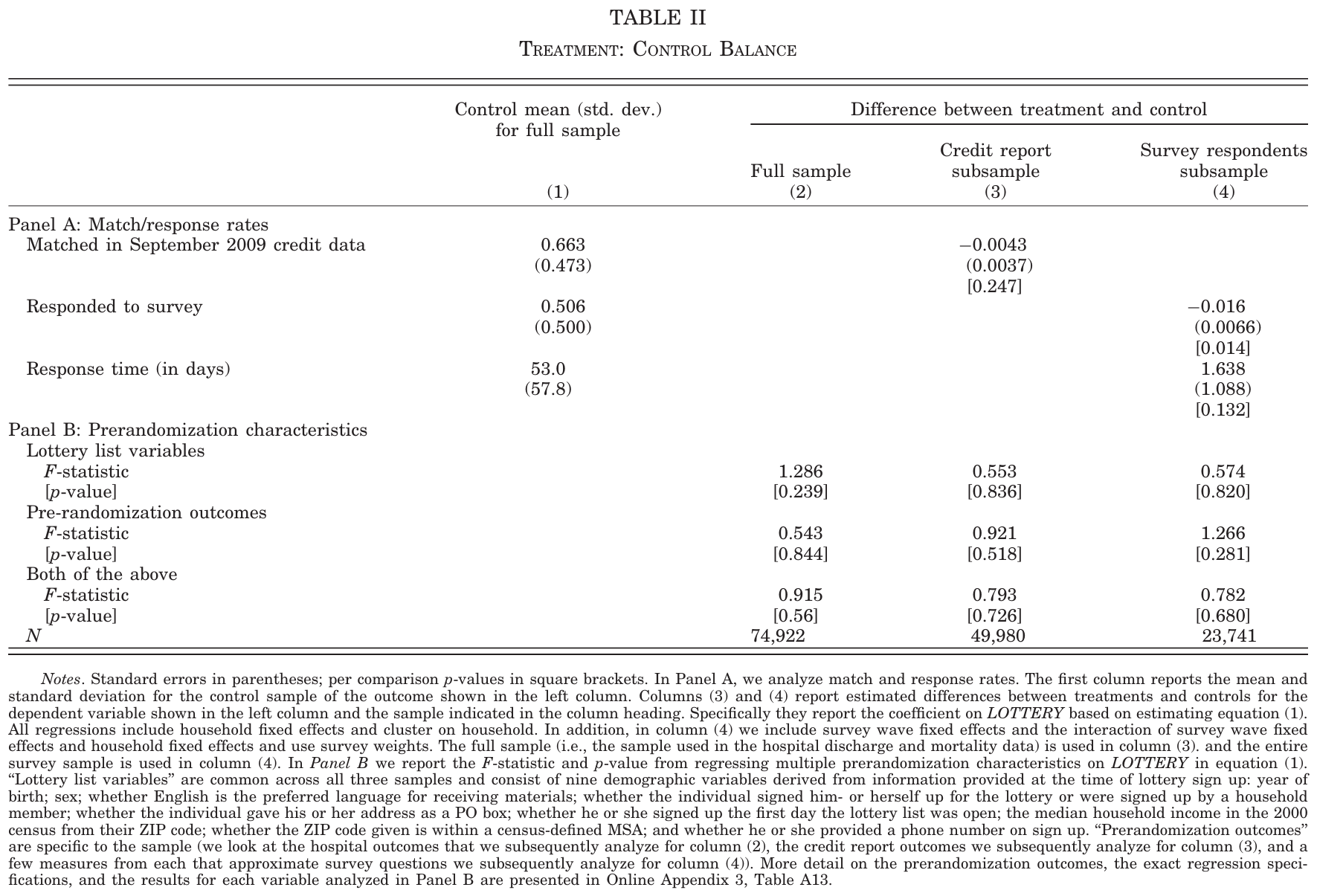
Explain what Table II tests. Compare the match and response rates in Panel A and the joint balance tests in Panel B. How does the evidence bear on the validity of the comparisons, particularly among survey respondents?
:::
{width=100%}
Read Panel A separately from Panel B. Similar measured baseline characteristics are reassuring about the observed samples. Selection into responding could still depend on unobserved outcomes. The paper discusses sensitivity to this concern.
### First stage: Table III
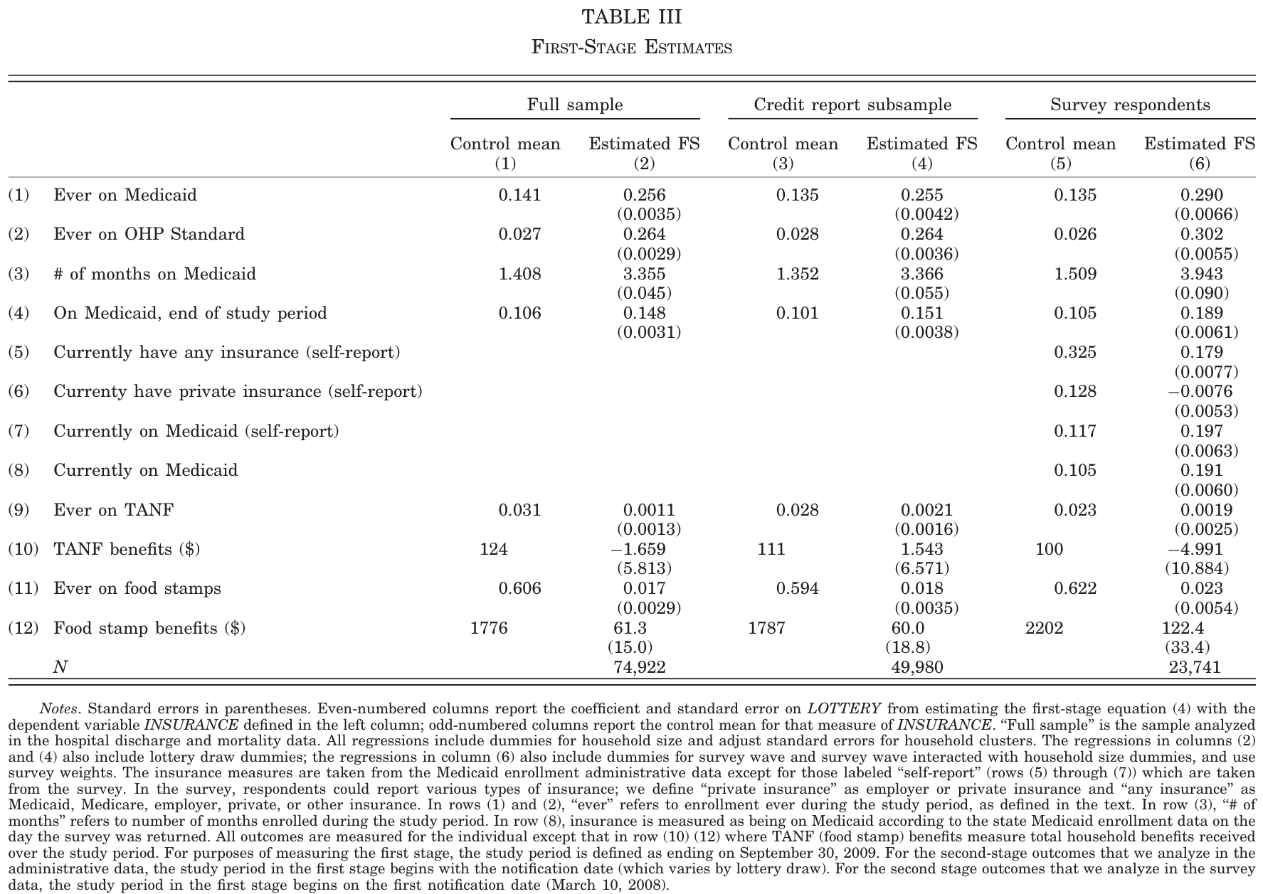
::: {.callout-note title="Your turn"}
Explain the first row of Table III, including the control mean, estimated first stage, units, and standard error. Why is the first stage less than one? Why might it differ across samples? Also consider the food-stamp results when assessing exclusion.
:::
{width=100%}
In the full sample, lottery selection raises the probability of ever having Medicaid during the study period by approximately **25.6 percentage points**. The comparable estimate among survey respondents is about **29 percentage points**. These are increases in enrolment associated with selection, rather than the enrolment rate of all lottery winners.
### The empirical specification
For the study's outcome equation, write
$$Y_i=\beta_0+\beta_1D_i+\sum_{k=1}^{K}\beta_{k+1}X_{ik}+u_i.$$
Lottery selection $Z_i$ instruments Medicaid coverage $D_i$. The authors estimate the **ITT** by regressing $Y_i$ on lottery selection and the relevant controls. They estimate the **first stage** by regressing Medicaid coverage on the same instrument and controls.
Three design details matter:
- **Household-list size:** when any listed household member won, the household could apply. Include indicators for the number of household members on the lottery list.
- **Survey design:** for survey outcomes, also include survey-wave indicators and their interactions with household-list-size indicators, and use the supplied survey weights. The exercise represents each observed combination with one categorical variable.
- **Inference:** cluster standard errors by household. This permits heteroskedasticity and correlation among people in the same household.
For administrative outcomes, the paper also includes lottery-draw indicators and, where available, the corresponding pre-randomisation outcome. Keep each reported outcome paired with the first stage for its own estimation sample and specification.
### Hospital use: Table IV
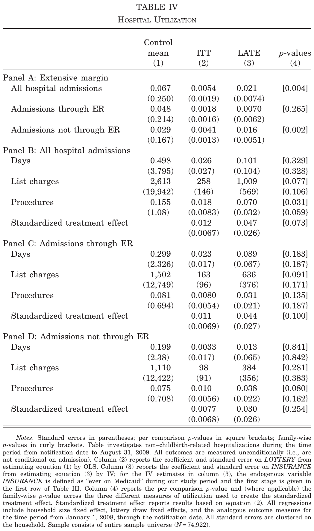
::: {.callout-note title="Your turn"}
Interpret Panel A of Table IV. Distinguish the control mean, ITT, and LATE. Convert the first row's effects into percentage points. What does the uncertainty permit you to conclude about admissions through the emergency room?
:::
{width=100%}
For any hospital admission, the reported ITT is 0.0054 and the LATE is approximately 0.021. The latter corresponds to a **2.1-percentage-point increase** in admission probability for the relevant compliers. The simple calculation $0.0054/0.256\simeq0.021$ illustrates the rescaling. Exact calculations use unrounded estimates and the same covariates and sample. Admissions through an emergency room are hospital admissions; they do not include every emergency-department visit.
### Survey health care use: Table V
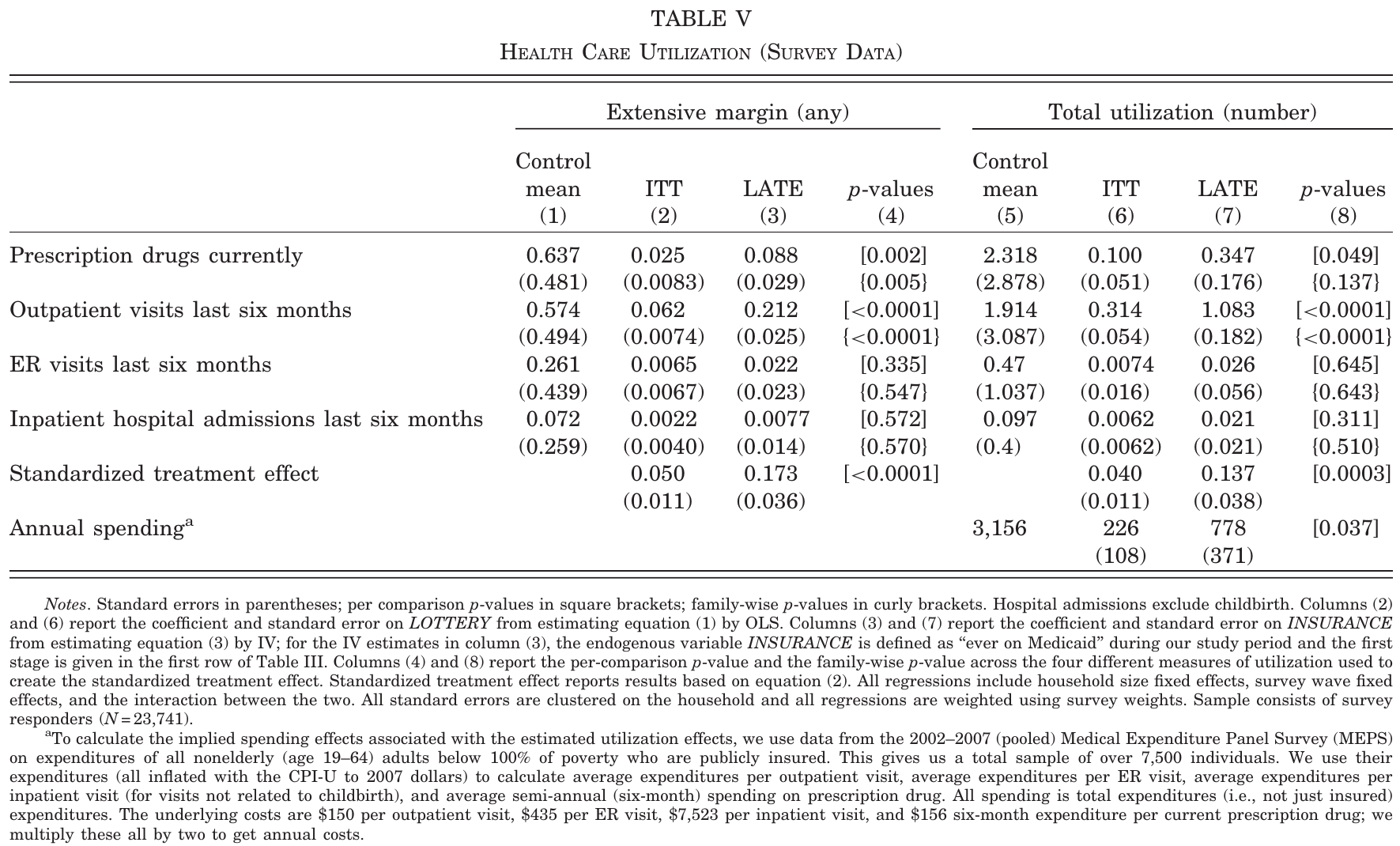
::: {.callout-note title="Your turn"}
Interpret the outpatient-visit row of Table V. Explain the difference between any visit and number of visits. Which first stage from Table III belongs with the survey results? What is the estimated effect of Medicaid on the probability of any outpatient visit?
:::
{width=100%}
The reported ITT for any outpatient visit is about **6.2 percentage points**, and the LATE is about **21.2 percentage points**. The after-class exercise estimates this relationship from the public survey files.
### Financial strain: Table VIII
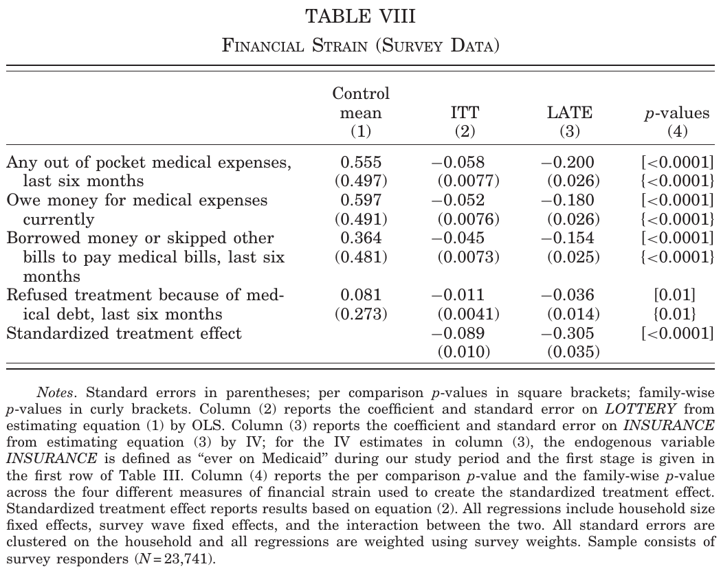
::: {.callout-note title="Your turn"}
Interpret the effects in Table VIII. Use at least two outcomes, discussing magnitude and uncertainty. Why might a change in out-of-pocket spending or medical debt matter for evaluating health insurance?
:::
{width=100%}
### Health and external validity: Table IX
::: {.callout-note title="Your turn"}
Explain the evidence on health in Table IX. Distinguish the administrative outcome from self-reported outcomes, and distinguish imprecise estimates from evidence of a small effect. Whose treatment effect is estimated, and how far would you generalise the findings to another insurance expansion?
:::
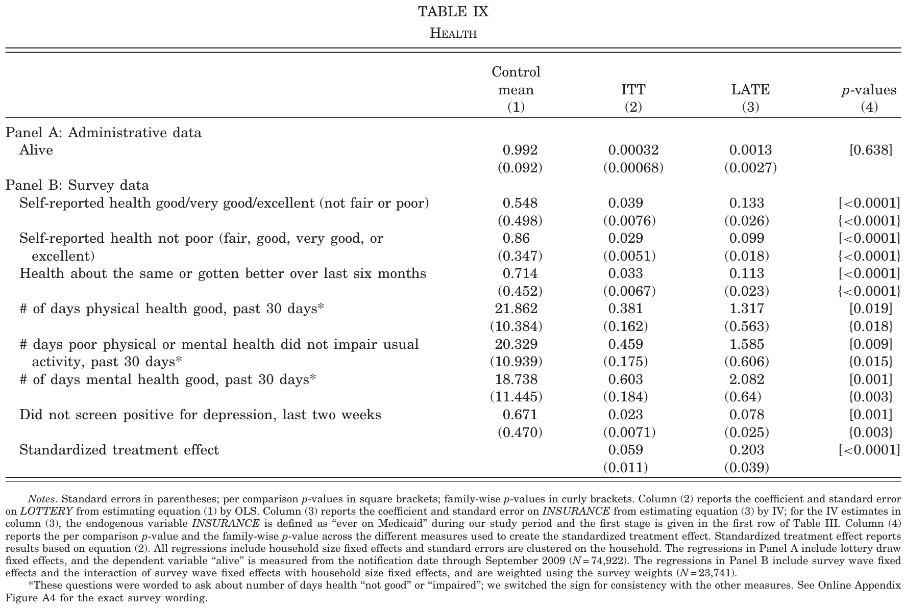{width=100%}
The population entered a waiting list for a particular programme in a particular setting. The IV estimate applies to people whose Medicaid coverage was changed by the lottery. Generalising requires considering eligibility, existing access to care, the insurance package, provider capacity, and the follow-up period.
### Assessing the IV assumptions
The lottery provides the basis for independence conditional on household-list size. The first-stage estimates establish relevance. Monotonicity asks whether winning could cause someone to lose Medicaid coverage that they would otherwise have obtained. Exclusion asks whether selection affects outcomes through any route other than the Medicaid coverage being instrumented.
Table III also reports changes in food-stamp receipt. Consider whether assistance with applications or information could influence other programmes directly, or whether other-programme use changes as a consequence of obtaining Medicaid. A downstream consequence of Medicaid can be part of its total effect; a separate pathway from the lottery to an outcome raises an exclusion concern. Similarly, effects on a person's outcome through another household member's coverage need attention when interpreting an IV for the person's own coverage.
**Internal validity** concerns the credibility of the causal interpretation for the study's comparison. **External validity** concerns the applicability of that effect to other populations, policies, and settings.
## 8. After class
The [ungraded exercise](../exercises/03-iv-late.qmd) asks you to estimate the first stage, the ITT, and a 2SLS effect for outpatient use; verify the ratio relationship; and interpret the result for compliers. Use Quarto to keep the code, output, and explanation together.
## References
- Angrist, J. D., and A. B. Krueger (2001). “Instrumental Variables and the Search for Identification: From Supply and Demand to Natural Experiments.” *Journal of Economic Perspectives* 15(4): 69–85. [DOI](https://doi.org/10.1257/jep.15.4.69).
- Angrist, J. D., and J.-S. Pischke (2009). *Mostly Harmless Econometrics: An Empiricist's Companion*. Princeton University Press, Chapter 4. [Book](https://www.mostlyharmlesseconometrics.com/).
- Angrist, J. D., and J.-S. Pischke (2015). *Mastering 'Metrics: The Path from Cause to Effect*. Princeton University Press, Chapter 3. [Companion resources](https://www.masteringmetrics.com/online-metrics-resources/mastering-iv/).
- Cunningham, S. *Causal Inference: The Remix*. Online edition, Chapter 7. [Chapter](https://mixtape.scunning.com/07-instrumental_variables).
- Finkelstein, A., S. Taubman, B. Wright, M. Bernstein, J. Gruber, J. P. Newhouse, H. Allen, K. Baicker, and the Oregon Health Study Group (2012). “The Oregon Health Insurance Experiment: Evidence from the First Year.” *Quarterly Journal of Economics* 127(3): 1057–1106. [DOI](https://doi.org/10.1093/qje/qjs020).
- Huntington-Klein, N. *The Effect: An Introduction to Research Design and Causality*. Online edition, Chapter 19. [Chapter](https://theeffectbook.net/ch-InstrumentalVariables.html).
- Imbens, G. W., and J. D. Angrist (1994). “Identification and Estimation of Local Average Treatment Effects.” *Econometrica* 62(2): 467–475. [DOI](https://doi.org/10.2307/2951620).








