Instrumental Variables and LATE

PP5001 · Week 3

Professor David A. Jaeger

Recall: Omitted Variables Bias

The true population relationship is

Y_i=\beta_0+\beta_1D_i+\beta_2A_i+\nu_i,

where Y_i is earnings, D_i is years of schooling, and A_i is ability. \beta_1 is the causal effect of an additional year of schooling.

Recall the population regression of ability on schooling:

A_i=\gamma_0+\gamma_1D_i+v_i.

Omitting ability gives a short-regression slope of

\beta_1^{S}=\beta_1+\beta_2\gamma_1.

If ability raises earnings and is positively related to schooling, the short regression overstates the causal effect of schooling.

Omitted Variables Bias: The DAG

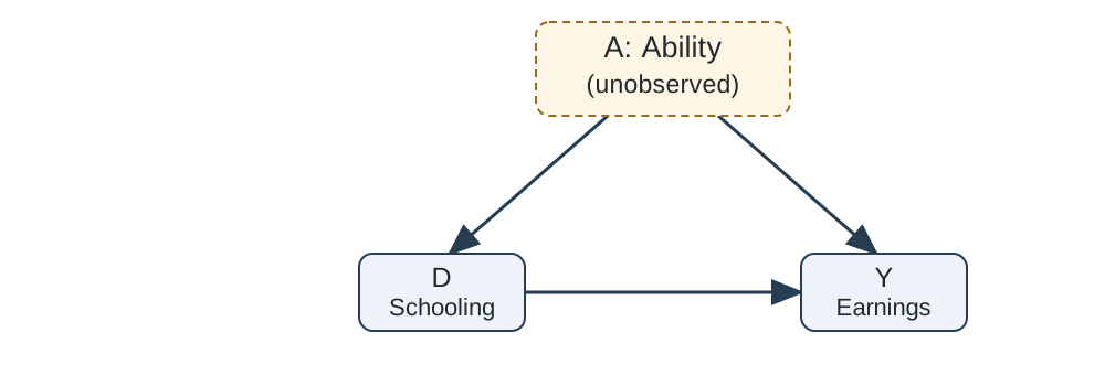
Ability affects both schooling and earnings, creating the backdoor path D\leftarrow A\rightarrow Y.

Our simple regression combines the causal effect along D\rightarrow Y with the association arising through unobserved ability.

Bias and Unbiasedness of OLS

Across repeated samples, the estimated slope varies. Its bias is

\operatorname{Bias}\left(\widehat\beta_1^{S}\right)=E\left[\widehat\beta_1^{S}\right]-\beta_1.

Imagine repeatedly observing outcomes for the same schooling values, \mathbf D=\left(D_1,\ldots,D_n\right). From Y_i=\beta_0+\beta_1D_i+u_i,

\widehat\beta_1^{S}=\beta_1+\frac{\sum_i\left(D_i-\overline D\right)u_i}{\sum_i\left(D_i-\overline D\right)^2}.

Conditional on \mathbf D, the schooling values and denominator are fixed:

E\left[\widehat\beta_1^{S}\mid\mathbf D\right]=\beta_1+ \frac{\sum_i\left(D_i-\overline D\right)E\left[u_i\mid\mathbf D\right]}{\sum_i\left(D_i-\overline D\right)^2}.

If E\left[u_i\mid\mathbf D\right]=0, OLS is unbiased. When omitted ability is related to schooling, this condition generally fails.

Omitted Ability and the Bias of OLS

Substitute u_i=\beta_2A_i+\nu_i and assume E\left[\nu_i\mid\mathbf D\right]=0:

E\left[\widehat\beta_1^{S}\mid\mathbf D\right]=\beta_1+\beta_2 \frac{\sum_i\left(D_i-\overline D\right)E\left[A_i\mid\mathbf D\right]}{\sum_i\left(D_i-\overline D\right)^2}.

Now assume the conditional mean of ability is linear in schooling:

E\left[A_i\mid\mathbf D\right]=\gamma_0+\gamma_1D_i.

Since \sum_i\left(D_i-\overline D\right)=0, the numerator becomes

\sum_i\left(D_i-\overline D\right)\left(\gamma_0+\gamma_1D_i\right) =\gamma_1\sum_i\left(D_i-\overline D\right)^2.

Hence, using the population slope of the ability-on-schooling regression,

E\left[\widehat\beta_1^{S}\mid\mathbf D\right] =\beta_1+\beta_2\gamma_1 =\beta_1+\beta_2\frac{\operatorname{Cov}\left(A_i,D_i\right)}{\operatorname{Var}\left(D_i\right)}.

What can we do if ability is unobserved?

The Wald Estimator: Setup

Write Y_i=\beta_0+\beta_1D_i+u_i, where u_i=\beta_2A_i+\nu_i.

Suppose we have a binary instrument, Z_i, that has two properties at the same time:

E\left[u_i\mid Z_i=1\right]=E\left[u_i\mid Z_i=0\right]=0,

E\left[D_i\mid Z_i=1\right]\ne E\left[D_i\mid Z_i=0\right].

The instrument shifts schooling and affects earnings through schooling.

We call the first relationship the orthogonality assumption and the second relationship the relevance assumption.

Finding a variable with either property is easy. The challenge is finding one that satisfies both at the same time: it predicts years of schooling while remaining uncorrelated with the unobserved determinants of earnings.

The Instrument in the DAG

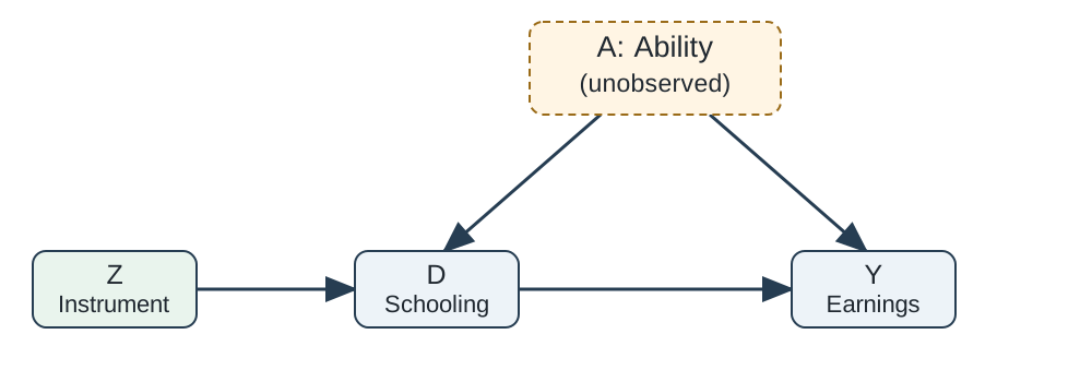
• Relevance: Z\rightarrow D shifts schooling.
• Exclusion: the effect of Z on earnings operates through schooling.
• Independence: Z is independent of ability and the other unobserved determinants of earnings.

The last two conditions support the orthogonality assumption.

Deriving the Wald Estimator

Taking conditional expectations of the outcome equation:

\begin{aligned} E\left[Y_i\mid Z_i=1\right]&=\beta_0+\beta_1E\left[D_i\mid Z_i=1\right],\\ E\left[Y_i\mid Z_i=0\right]&=\beta_0+\beta_1E\left[D_i\mid Z_i=0\right]. \end{aligned}

Subtract the second equation from the first:

\underbrace{E\left[Y_i\mid Z_i=1\right]-E\left[Y_i\mid Z_i=0\right]}_{\text{difference in outcomes}} =\beta_1\underbrace{\left[E\left[D_i\mid Z_i=1\right]-E\left[D_i\mid Z_i=0\right]\right]}_{\text{difference in treatment}}.

Solve for \beta_1 and use the analogy principle to replace the population conditional means with the sample conditional means:

\widehat\beta_{1,\mathrm{Wald}}= \frac{\overline{Y}_{Z=1}-\overline{Y}_{Z=0}} {\overline{D}_{Z=1}-\overline{D}_{Z=0}}.

An Illustrative Schooling and Earnings Model

Generate 400 observations from these relationships:

D_i=11+5Z_i+1.8A_i+v_i,\qquad Y_i=100+5D_i+20A_i+\nu_i.

Z_i is binary with probability 1/2. Ability A_i and the disturbances v_i,\nu_i are independent, mean-zero normal variables with standard deviations 1, 0.65, and 10; all are independent of Z_i.

The true schooling effect is 5. Ability raises both schooling and earnings:

\operatorname{Cov}\left(A_i,D_i\right)=1.8,\qquad \operatorname{Var}\left(D_i\right)=25\left(0.25\right)+1.8^2+0.65^2=9.9125.

The population short-regression slope is therefore

\beta_1^S=5+20\frac{1.8}{9.9125}\approx8.63.

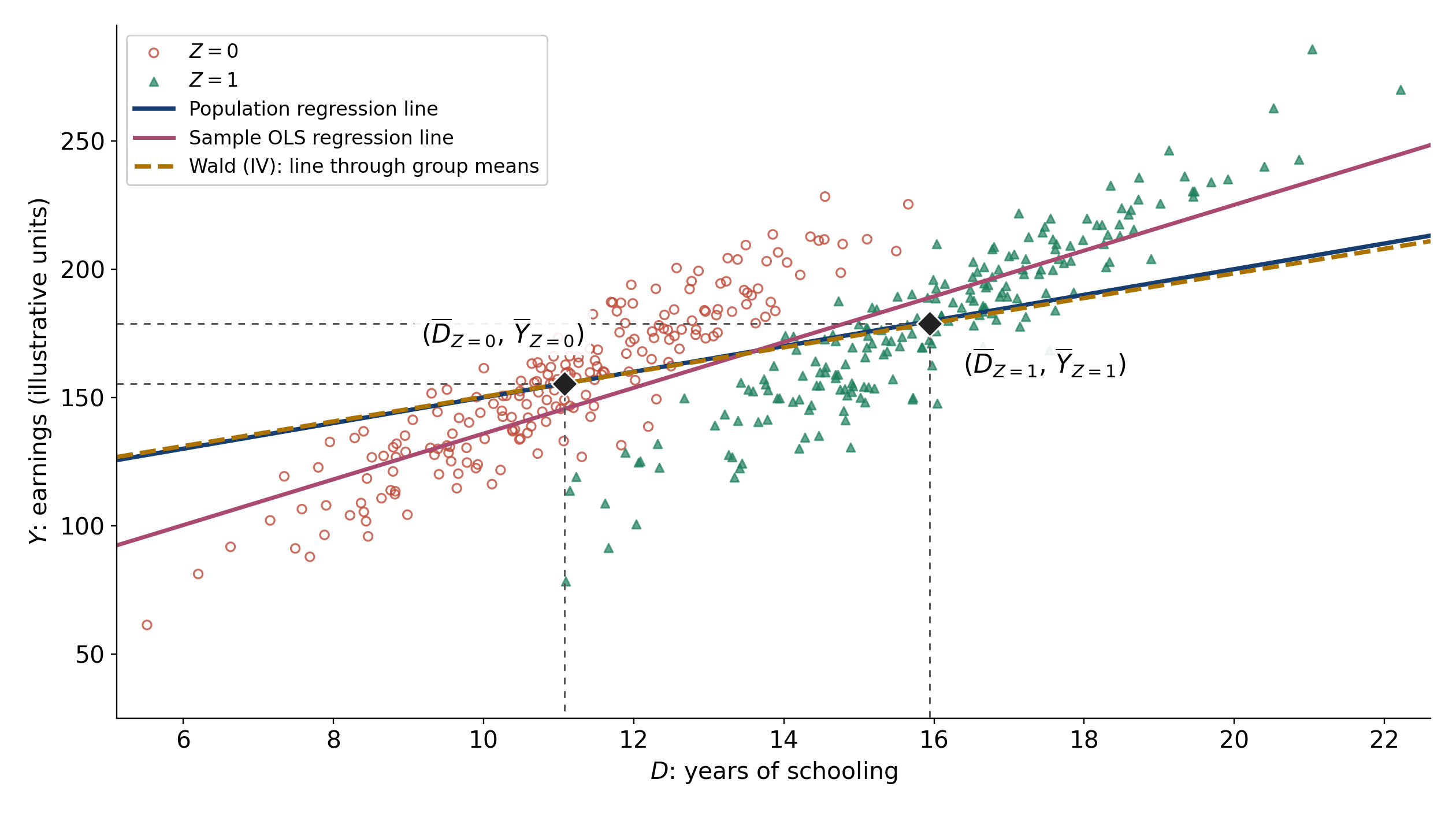
Omitting ability gives an upward bias of approximately 3.63. The graph shows the sample OLS and Wald estimates alongside the true relationship.

The Wald Estimator: A Graphical Illustration

Understanding the Wald Estimator

• Population regression line: the true causal slope is \beta_1=5.
• Sample OLS regression line: omitted ability affects both D_i and Y_i, making the estimated slope too steep in this example.
• Instrument groups: open circles have Z_i=0; triangles have Z_i=1.
• Wald (IV) line: passes through the two group means, \left(\overline{D}_{Z=0},\overline{Y}_{Z=0}\right) and \left(\overline{D}_{Z=1},\overline{Y}_{Z=1}\right).

\text{Slope of IV line}=\frac{\overline{Y}_{Z=1}-\overline{Y}_{Z=0}}{\overline{D}_{Z=1}-\overline{D}_{Z=0}}=\frac{\text{vertical difference between means}}{\text{horizontal difference between means}}.

The instrument shifts D_i independently of ability. Sampling variation means that the IV line need not coincide exactly with the population line.

First Stage and Reduced Form: Terminology

• First stage: regress the endogenous explanatory variable on all the exogenous variables.
• Reduced form: regress the outcome on all the exogenous variables.

Both include the excluded instrument(s) and any included exogenous covariates, together with an intercept.

The term reduced form comes from simultaneous-equations models: we solve the system to express each endogenous variable as a function of all the exogenous variables and a disturbance.

In IV applications, we call the equation for Y_i “the reduced form.” The equation for D_i, which we call the first stage, is also a reduced-form equation.

In our simplest example, both regressions use an intercept and Z_i.

First Stage and Reduced Form

\begin{aligned} D_i&=\pi_0+\pi_1Z_i+v_i &&\text{First stage}\\ Y_i&=\delta_0+\delta_1Z_i+e_i &&\text{Reduced form} \end{aligned}

For a binary instrument:

\pi_1=E\left[D_i\mid Z_i=1\right]-E\left[D_i\mid Z_i=0\right], \delta_1=E\left[Y_i\mid Z_i=1\right]-E\left[Y_i\mid Z_i=0\right].

With one endogenous explanatory variable and one excluded instrument, the model is exactly identified. The IV estimate is the ratio of their reduced-form and first-stage coefficients:

\widehat\beta_{1,\mathrm{Wald}}=\frac{\widehat\delta_1}{\widehat\pi_1}.

From Wald to the IV Estimator

For binary Z_i, with P\left(Z_i=1\right)=p,

\begin{aligned} \operatorname{Cov}\left(Y_i,Z_i\right)&=\left[E\left[Y_i\mid Z_i=1\right]-E\left[Y_i\mid Z_i=0\right]\right]p\left(1-p\right),\\ \operatorname{Cov}\left(D_i,Z_i\right)&=\left[E\left[D_i\mid Z_i=1\right]-E\left[D_i\mid Z_i=0\right]\right]p\left(1-p\right). \end{aligned}

The common factor cancels, giving

\beta_1=\frac{\operatorname{Cov}\left(Y_i,Z_i\right)}{\operatorname{Cov}\left(D_i,Z_i\right)} =\frac{\operatorname{Cov}\left(Y_i,Z_i\right)/\operatorname{Var}\left(Z_i\right)}{\operatorname{Cov}\left(D_i,Z_i\right)/\operatorname{Var}\left(Z_i\right)}.

This is the reduced-form slope divided by the first-stage slope. The covariance expression also applies to a continuous instrument with \operatorname{Cov}\left(Z_i,u_i\right)=0 and a nonzero first stage.

IV as a Method-of-Moments Estimator

Orthogonality concerns the covariance between the instrument and the outcome disturbance:

\begin{aligned} 0&=\operatorname{Cov}\left(Z_i,u_i\right)\\ &=E\left[\left(Z_i-E\left[Z_i\right]\right)\left(u_i-E\left[u_i\right]\right)\right]\\ &=E\left[\left(Z_i-E\left[Z_i\right]\right)u_i\right]. \end{aligned}

The “useful result” lets us drop the mean from the second term because E\left[Z_i-E\left[Z_i\right]\right]=0.

Now substitute u_i=Y_i-\beta_0-\beta_1D_i:

E\left[\left(Z_i-E\left[Z_i\right]\right) \left(Y_i-\beta_0-\beta_1D_i\right)\right]=0.

IV by Method of Moments: The Sample Estimator

Use the analogy principle to replace population moments with sample moments:

\frac{1}{n}\sum_i\left(Z_i-\overline Z\right) \left(Y_i-\widehat\beta_0-\widehat\beta_1D_i\right)=0.

Since \sum_i\left(Z_i-\overline Z\right)=0, the intercept drops out. Solving gives

\widehat\beta_{1,\mathrm{IV}}= \frac{\sum_i\left(Z_i-\overline Z\right)\left(Y_i-\overline Y\right)} {\sum_i\left(Z_i-\overline Z\right)\left(D_i-\overline D\right)} =\frac{\widehat{\operatorname{Cov}}\left(Z_i,Y_i\right)} {\widehat{\operatorname{Cov}}\left(Z_i,D_i\right)}.

This is the method of moments: choose the coefficients to satisfy the sample counterpart of the population condition. With a binary instrument, it gives the Wald estimator; the formula also applies to a continuous instrument.

Using the Instrument to Predict Treatment

Our goal is to isolate variation in D_i that is uncorrelated with u_i.

The population first-stage regression gives the instrument-predicted component:

D_i^*=\pi_0+\pi_1Z_i,\qquad \pi_1=\frac{\operatorname{Cov}\left(D_i,Z_i\right)}{\operatorname{Var}\left(Z_i\right)}.

Because D_i^* is a linear function of the instrument,

\operatorname{Cov}\left(D_i^*,u_i\right)=\pi_1\operatorname{Cov}\left(Z_i,u_i\right)=0.

We estimate this component using the fitted values

\widehat D_i=\widehat\pi_0+\widehat\pi_1Z_i.

Dividing Schooling into Two Components

The first-stage regression decomposes observed schooling exactly:

D_i=\underbrace{\widehat D_i}_{\text{exogenous part}} +\underbrace{\widehat v_i}_{\text{endogenous part}},\qquad \widehat v_i=D_i-\widehat D_i.

• \widehat D_i=\widehat\pi_0+\widehat\pi_1Z_i: schooling predicted by the instrument. A valid instrument isolates variation that is unrelated to the unobserved determinants of earnings.
• \widehat v_i: the first-stage residual. It contains the remaining variation in schooling, including variation associated with unobserved ability.

The population counterpart is D_i=D_i^*+v_i. Instrument validity implies

\operatorname{Cov}\left(D_i^*,u_i\right)=0,\qquad \operatorname{Cov}\left(D_i,u_i\right)=\operatorname{Cov}\left(v_i,u_i\right).

IV uses the instrument-predicted component to estimate the causal effect of schooling.

Instrumental Variables as Two-Stage Least Squares

First stage: regress D_i on an intercept and Z_i; obtain \widehat D_i.

Second stage: regress Y_i on an intercept and \widehat D_i.

Y_i=\widehat\beta_{0,\mathrm{2SLS}}+\widehat\beta_{1,\mathrm{2SLS}}\widehat D_i+\widehat r_i.

Here \widehat r_i is the residual from this regression.

With a binary instrument, \widehat D_i=\overline{D}_{Z=0} for the first group and \widehat D_i=\overline{D}_{Z=1} for the second. The second-stage slope is therefore the slope through the two group means:

\widehat\beta_{1,\mathrm{2SLS}}= \frac{\overline{Y}_{Z=1}-\overline{Y}_{Z=0}}{\overline{D}_{Z=1}-\overline{D}_{Z=0}} =\widehat\beta_{1,\mathrm{Wald}}.

This is the graphical argument expressed as two regressions.

Including Covariates

\begin{aligned} Y_i&=\beta_0+\beta_1D_i+\sum_{k=1}^{K}\beta_{k+1}X_{ik}+u_i,\\ D_i&=\pi_0+\pi_1Z_i+\sum_{k=1}^{K}\pi_{k+1}X_{ik}+v_i. \end{aligned}

Here X_{ik} is covariate k for person i, and K is the number of covariates. Include the same exogenous covariates in both stages.

With one excluded instrument, 2SLS equals the reduced-form coefficient divided by the first-stage coefficient when the regressions use the same observations, weights, and covariates.

In Oregon, indicators for the number of household members on the lottery list are part of the identifying comparison.

Estimating IV in Python

import linearmodels.iv as iv

model = iv.IV2SLS.from_formula(
    "outcome ~ 1 + [insured ~ selected]", data=df
)
result = model.fit(cov_type="robust")

[insured ~ selected] instruments insurance with lottery selection; 1 includes an intercept.

Use the IV routine’s standard errors. Running two OLS regressions manually reproduces the coefficient, but the second regression’s ordinary standard errors are incorrect for IV.

With a binary outcome, this is a linear probability model. Interpret coefficients in probability units, and multiply by 100 for percentage points.

Finite Samples and Consistency

Unbiasedness concerns the mean of an estimator across repeated samples of a given size: E\left[\widehat\beta_1\right]=\beta_1.

Consistency concerns what happens as the sample size grows: the probability that the estimate is close to the true parameter approaches one.

For one instrument, the IV estimator is

\widehat\beta_{1,\mathrm{IV}}=\beta_1+ \frac{n^{-1}\sum_i\left(Z_i-\overline Z\right)u_i} {n^{-1}\sum_i\left(Z_i-\overline Z\right)D_i}.

With independent random sampling and finite second moments, the numerator converges to \operatorname{Cov}\left(Z_i,u_i\right)=0, and the denominator to \operatorname{Cov}\left(Z_i,D_i\right)\ne0. Hence

\widehat\beta_{1,\mathrm{IV}}\xrightarrow{p}\beta_1.

IV can be consistent without being unbiased in finite samples. We return to its finite-sample behaviour when studying weak instruments.

Heterogeneous Treatment Effects

So far, \beta_1 has been a constant effect. Now allow

Y_i^1-Y_i^0

to differ across people.

Health insurance might have different effects for people with different health needs or access to care.

For whom does IV estimate an average treatment effect?

The answer depends on whose treatment status the instrument changes.

Potential Treatment Statuses

• D_i^1: treatment status if the instrument equals one.
• D_i^0: treatment status if the instrument equals zero.

D_i=Z_iD_i^1+\left(1-Z_i\right)D_i^0.

The superscript on Y_i^d denotes the treatment state.

The superscript on D_i^z denotes the instrument state.

For Oregon, imagine each person’s Medicaid enrolment with and without the lottery offer.

Four Responses to the Instrument

Type	D_i^0	D_i^1	Response
Never-taker	0	0	No treatment under either assignment
Complier	0	1	Treatment when offered
Always-taker	1	1	Treatment under either assignment
Defier	1	0	Treatment only without the offer

These types are defined relative to a particular instrument.

We observe only one potential treatment status for each person. A treated lottery winner could be an always-taker or a complier.

Assumption 1: Instrument Independence

The instrument is independent of potential outcomes and treatment statuses:

Z_i\perp\left(Y_i^0,Y_i^1,D_i^0,D_i^1\right).

Random assignment of an offer can support this assumption.

In observational applications, we need to explain why the instrument supplies an as-good-as-random comparison, possibly conditional on covariates.

The derivation first considers unconditional independence. In Oregon, independence is conditional on household-list size.

Assumption 2: Exclusion

Let Y_i\left(d,z\right) denote an outcome under treatment d and instrument value z.

Exclusion requires

Y_i\left(d,1\right)=Y_i\left(d,0\right)=Y_i^d.

The instrument affects the outcome through treatment. We can then write

Y_i=Y_i^0+\left(Y_i^1-Y_i^0\right)D_i.

For Oregon: could winning affect health care use or well-being through a route other than obtaining Medicaid?

Assumption 3: Monotonicity

Orient the instrument so it encourages treatment. Assume

D_i^1\ge D_i^0\qquad\text{for every }i.

The instrument increases treatment for compliers and leaves treatment unchanged for always-takers and never-takers. There are no defiers.

For Oregon: could winning cause someone to lose Medicaid coverage they would otherwise have obtained?

The assumption concerns each person’s response to the instrument, beyond its average first-stage effect.

Assumption 4: Relevance

The instrument must change the probability of treatment:

E\left[D_i\mid Z_i=1\right]-E\left[D_i\mid Z_i=0\right]>0.

Under independence and monotonicity, this difference is the proportion of compliers.

If the instrument changes nobody’s treatment, it supplies no treatment comparison.

As in Week 1, we assume that treatment is well defined and that one person’s outcome does not depend on other people’s treatment assignments (SUTVA).

The LATE Theorem

For binary treatment and a binary instrument, under independence, exclusion, monotonicity (D_i^1\ge D_i^0), and relevance,

\frac{E\left[Y_i\mid Z_i=1\right]-E\left[Y_i\mid Z_i=0\right]} {E\left[D_i\mid Z_i=1\right]-E\left[D_i\mid Z_i=0\right]} =E\left[Y_i^1-Y_i^0\mid D_i^1>D_i^0\right] =\tau_{\mathrm{LATE}}.

The Wald ratio identifies the average treatment effect for compliers: people whose treatment status is changed by the instrument.

Imbens and Angrist (1994). We now prove the result.

Proof of LATE (1)

\begin{aligned} E\left[Y_i\mid Z_i=1\right] &=E\left[Y_i^0+\left(Y_i^1-Y_i^0\right)D_i\mid Z_i=1\right]\\ &=E\left[Y_i^0+\left(Y_i^1-Y_i^0\right)D_i^1\right]. \end{aligned}

The first equality uses exclusion: Z_i affects Y_i through treatment. The second uses D_i=D_i^1 when Z_i=1 and independence to remove the conditioning on Z_i.

Similarly,

\begin{aligned} E\left[Y_i\mid Z_i=0\right] &=E\left[Y_i^0+\left(Y_i^1-Y_i^0\right)D_i\mid Z_i=0\right]\\ &=E\left[Y_i^0+\left(Y_i^1-Y_i^0\right)D_i^0\right]. \end{aligned}

Therefore the numerator of the Wald ratio is

E\left[Y_i\mid Z_i=1\right]-E\left[Y_i\mid Z_i=0\right] =E\left[\left(Y_i^1-Y_i^0\right)\left(D_i^1-D_i^0\right)\right].

Proof of LATE (2)

Monotonicity implies that D_i^1-D_i^0 can equal zero or one. It excludes -1 as a possible value.

• For compliers, D_i^1-D_i^0=1.
• For always-takers and never-takers, D_i^1-D_i^0=0.

The product is zero for everyone except compliers. Its population mean is therefore the mean effect for compliers multiplied by their population share:

\begin{aligned} &E\left[\left(Y_i^1-Y_i^0\right)\left(D_i^1-D_i^0\right)\right]\\ &\qquad=E\left[Y_i^1-Y_i^0\mid D_i^1>D_i^0\right] \,P\left(D_i^1>D_i^0\right). \end{aligned}

The outcome difference between the instrument groups equals the average effect for compliers multiplied by their share of the population.

Proof of LATE (3)

Now consider the denominator of the Wald ratio:

\begin{aligned} E\left[D_i\mid Z_i=1\right]-E\left[D_i\mid Z_i=0\right] &=E\left[D_i^1-D_i^0\right]\\ &=P\left(D_i^1>D_i^0\right). \end{aligned}

The first equality follows from independence.

The second follows from monotonicity: the change in treatment equals one for compliers and zero for everyone else.

The first stage is therefore the proportion of compliers. Relevance ensures this proportion is positive, so we can divide by it.

Proof of LATE (4)

Putting the numerator and denominator together,

\begin{aligned} &\frac{E\left[Y_i\mid Z_i=1\right]-E\left[Y_i\mid Z_i=0\right]} {E\left[D_i\mid Z_i=1\right]-E\left[D_i\mid Z_i=0\right]}\\[0.6em] &\qquad=\frac{E\left[Y_i^1-Y_i^0\mid D_i^1>D_i^0\right] \,P\left(D_i^1>D_i^0\right)}{P\left(D_i^1>D_i^0\right)}\\[0.6em] &\qquad=E\left[Y_i^1-Y_i^0\mid D_i^1>D_i^0\right]. \end{aligned}

The complier share cancels. The Wald ratio identifies the local average treatment effect.

The LATE Theorem: Proved

We have established the following result.

For binary treatment and a binary instrument, under independence, exclusion, monotonicity (D_i^1\ge D_i^0), and relevance,

\frac{E\left[Y_i\mid Z_i=1\right]-E\left[Y_i\mid Z_i=0\right]} {E\left[D_i\mid Z_i=1\right]-E\left[D_i\mid Z_i=0\right]} =E\left[Y_i^1-Y_i^0\mid D_i^1>D_i^0\right] =\tau_{\mathrm{LATE}}.

The Wald ratio identifies the average treatment effect for compliers: people whose treatment status is changed by the instrument.

“Local” refers to this group of compliers.

With conditional random assignment, the argument applies within covariate groups; 2SLS with group indicators combines those comparisons. The notes explain the weighting.

LATE, ATT, and External Validity

The ATT averages effects among those observed receiving treatment. Under monotonicity, recipients can include always-takers and compliers assigned the offer.

The LATE averages effects among compliers.

When there are no always-takers, random assignment and the LATE assumptions also allow IV to identify the ATT.

Different valid instruments can change treatment for different people. To generalise an IV result, consider who responds to the instrument and whether their effects are informative for the policy population.

The Oregon Health Insurance Experiment

For discussion

• Read Sections II and III.

• Explain the policy problem, the waiting list, the lottery, and what winning allowed a household to do.

• Distinguish lottery assignment from obtaining Medicaid coverage.

The Lottery and Medicaid Coverage

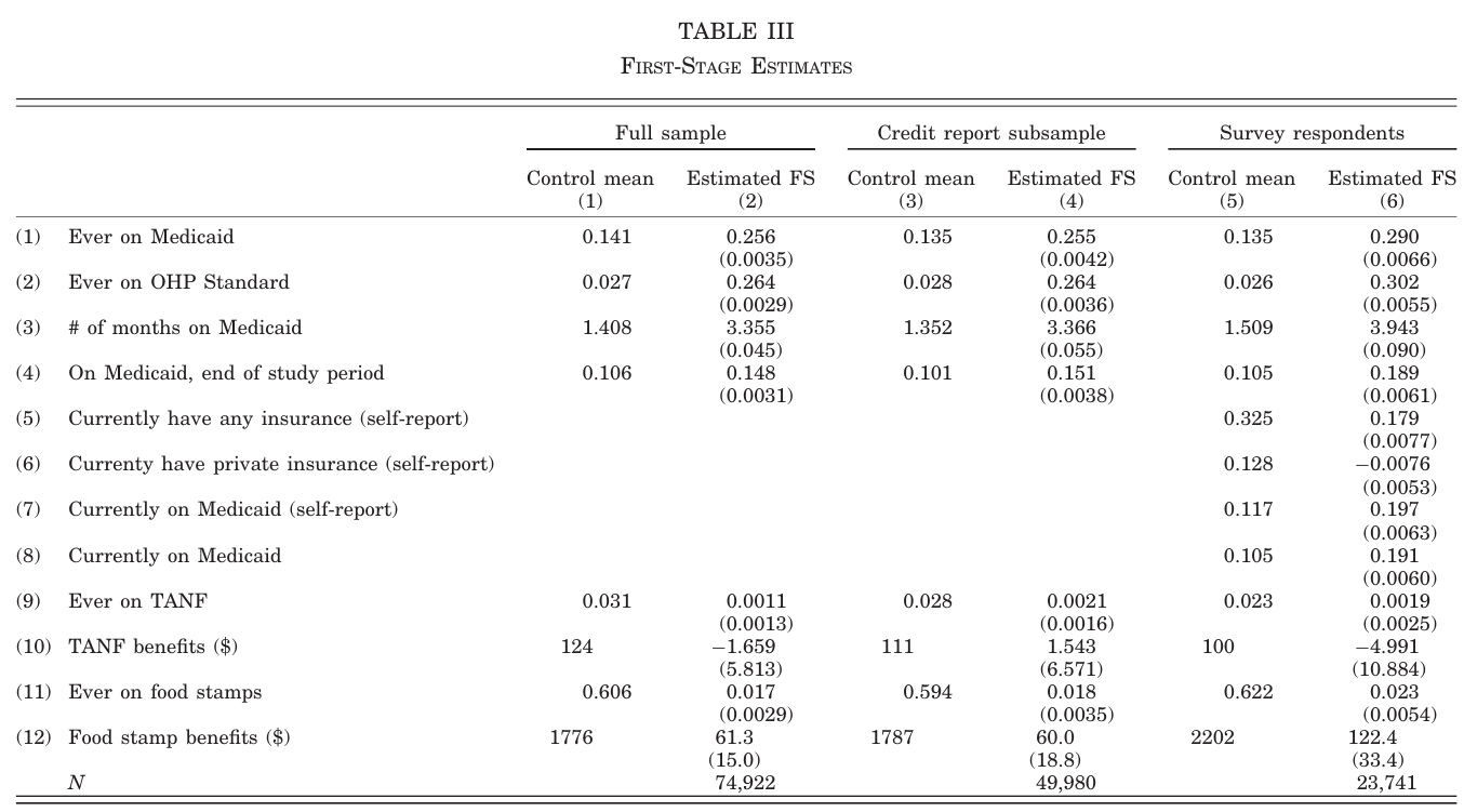
In 2008, Oregon used a lottery to offer people on a waiting list the opportunity to apply for OHP Standard.

Selected people still had to apply and meet eligibility requirements. Some enrolled; others did not. Some people in the control group obtained Medicaid through other routes.

The analysis sample contains 74,922 individuals, including 29,834 selected by the lottery.

The offer was assigned through the lottery. Medicaid enrolment reflects both the offer and people’s circumstances and choices.

Data

For discussion

• Read Section III.

• Identify the administrative and survey data and the outcomes each measures.

• Why do the analysis samples differ?

• Explain survey nonresponse and why it matters for the comparison.

Data Sources and Analysis Samples

• Lottery list: assignment, household-list size, and baseline characteristics.
• Administrative records: Medicaid enrolment, hospital use, credit reports, and mortality.
• Mail survey: health care use, financial strain, and self-reported health.

The effective weighted survey response rate was approximately 50%. The survey used intensive follow-up of a subsample of nonrespondents.

Different sources measure different outcomes and yield different analysis samples. Read the sample definitions and table notes.

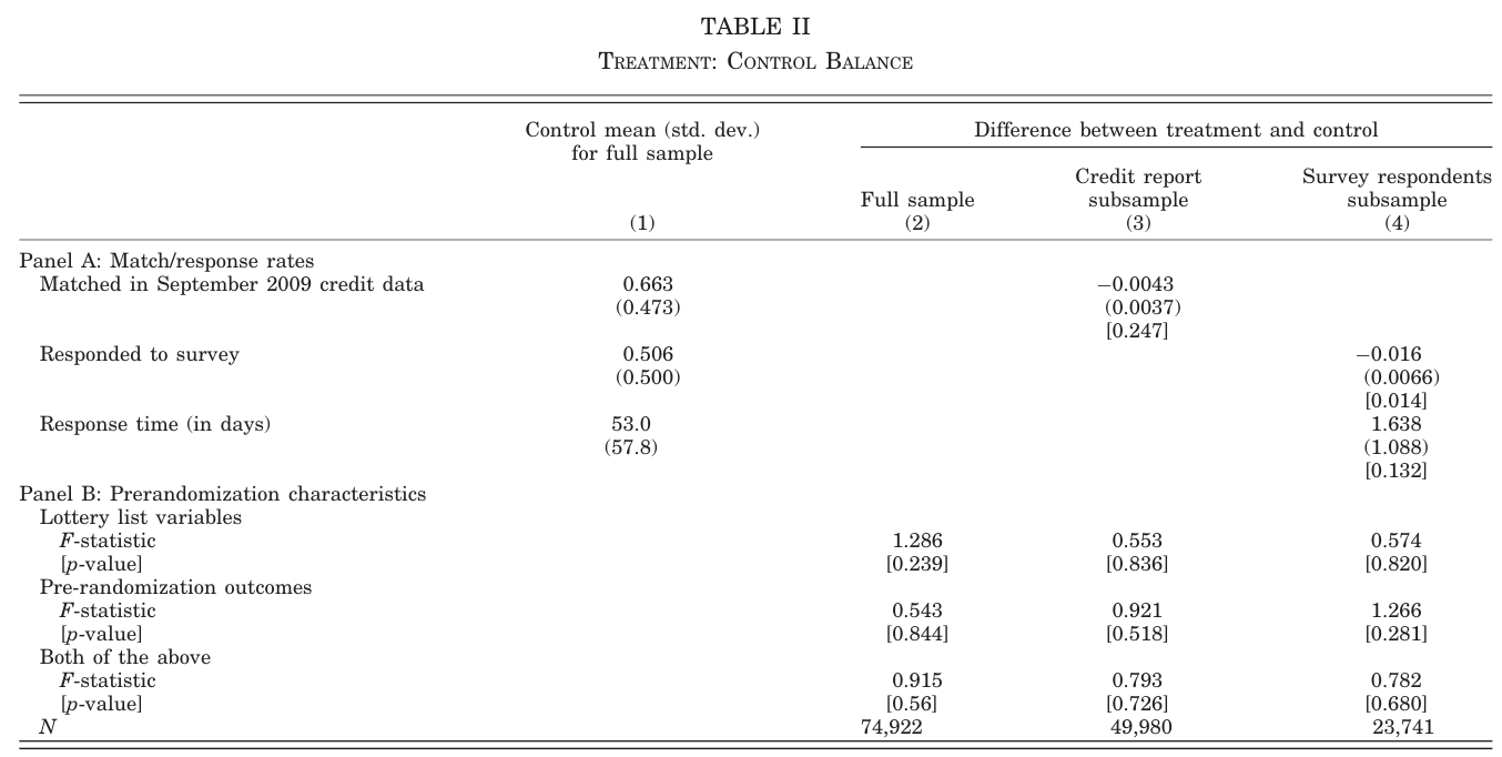
Balance: Table II

For discussion

First Stage: Table III

For discussion

Estimation in the Study

Lottery selection instruments Medicaid coverage.

• Include indicators for the number of household members on the lottery list: a household could apply if any listed member won.
• For survey outcomes, include survey-wave indicators and their interactions with household-list size, and use the survey weights.
• Cluster standard errors by household: allow heteroskedasticity and correlation among household members.

Use the same sample, controls, and weights for the reduced form and first stage when calculating their ratio.

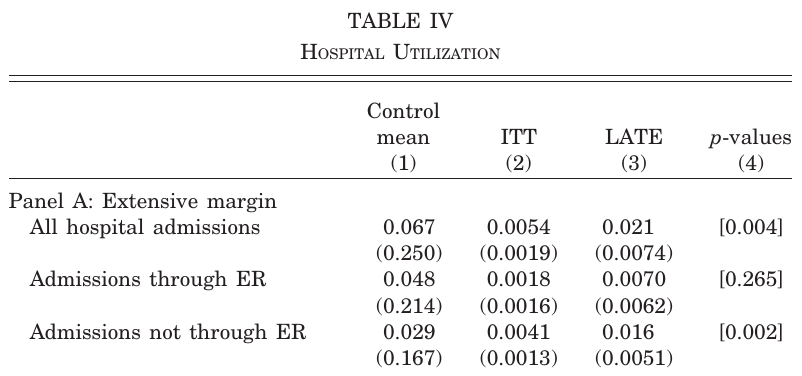
Hospital Use: Table IV, Panel A

For discussion

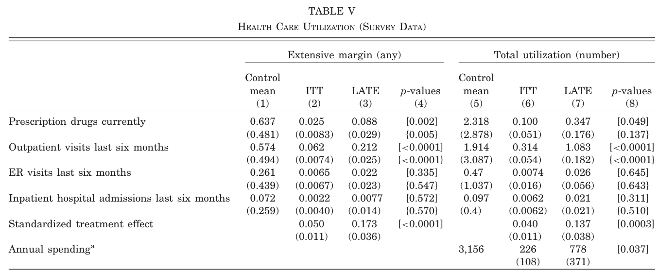
Health Care Use: Table V

For discussion

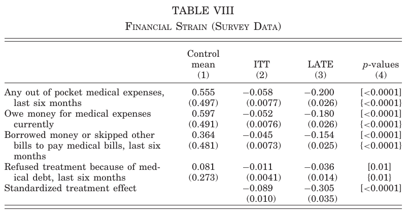
Financial Strain: Table VIII

For discussion

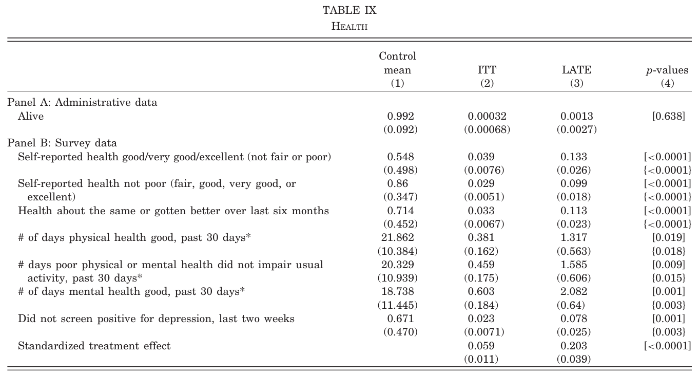
Health: Table IX

For discussion

Interpreting the Results

For discussion

• Bring together Tables IV, V, VIII, and IX.

• Whose effect does IV identify?

• What conclusions about the policy are supported?

External Validity

For discussion

• Explain what you would need to know before applying the Oregon findings to a different insurance expansion.

• Consider the population, take-up, follow-up period and scale of the expansion.

Assessing the IV Assumptions

Independence: lottery assignment, conditional on household-list size.

Relevance: lottery selection substantially increases Medicaid enrolment.

Exclusion: consider other routes from lottery selection to outcomes, including changes in other programme participation and other household members’ coverage.

Monotonicity: assess whether selection could reduce an individual’s Medicaid coverage.

Internal validity concerns the credibility of this causal comparison. External validity concerns its applicability to other populations and policies.

Recap: The IV Assumptions

In the linear model, the instrument must satisfy relevance and orthogonality: it predicts treatment and is uncorrelated with the outcome disturbance.

For a LATE interpretation, we require:

• Relevance: the instrument changes the probability of treatment.
• Independence: assignment of the instrument is independent of potential outcomes and potential treatment choices, conditional on the appropriate controls.
• Exclusion: the instrument affects the outcome only through treatment.
• Monotonicity: changing the instrument moves treatment in the same direction for everyone it affects; there are no defiers.

We also maintain SUTVA: well-defined treatment and no interference between individuals.

Next week: what features of judge and examiner assignment make each assumption credible?

After-Class Exercise

Use the Oregon public-use data to study outpatient visits.

1. Estimate the first stage and the ITT with the supplied design controls and weights.
2. Calculate their ratio and verify it with 2SLS.
3. Compare the estimate with Table V; interpret the effect, uncertainty, and complier population.

The exercise supplies data-import and estimation guidance. Work in Quarto. This practice is ungraded.

Exercise and Quarto setup file

References

• Finkelstein, A., et al. (2012). “The Oregon Health Insurance Experiment: Evidence from the First Year.” QJE 127(3): 1057–1106. Paper.
• Imbens, G. W., and J. D. Angrist (1994). “Identification and Estimation of Local Average Treatment Effects.” Econometrica 62(2): 467–475. Paper.
• Angrist, J. D., and A. B. Krueger (2001). “Instrumental Variables and the Search for Identification.” JEP 15(4): 69–85. Paper.
• Angrist and Pischke, Mastering ’Metrics, Chapter 3; Mostly Harmless Econometrics, Chapter 4.
• Huntington-Klein, The Effect, Chapter 19; Cunningham, Causal Inference: The Remix, Chapter 7.

Reading links and full references in the notes.