---
title: "Week 2: Matching"
subtitle: "Making an apples-to-apples comparison"
---
[Class slides](../slides/02-matching.qmd) · [Download slides as PDF](../resources/slides/02-matching.pdf) · [Problem Set 1](../exercises/02-matching.qmd) · [Download notes as PDF](../resources/notes/02-matching.pdf) · [Download Quarto source](../resources/sessions/02-matching.qmd)
Discussant assignments are available on Moodle. Prepare your assigned item individually; one person from each group will be called on to discuss it.
## Learning Objectives
By the end of this topic, you should be able to:
- Explain how LaLonde uses the experimental NSW result to assess estimates obtained with observational comparison groups.
- State the conditional independence and common support assumptions, and explain how matching aims to create an apples-to-apples comparison.
- Explain what a propensity score measures and use a logit model to estimate it.
- Estimate and interpret the ATT using inverse-probability-weighted regression, assess covariate balance, and compare the result with the experimental benchmark.
## Before class {#readings}
Read the notes and empirical readings below. We will start with the experimental evaluation of the National Supported Work demonstration by MDRC. The Week 2 practice is **Problem Set 1**, due **Friday 2 October 2026 at 12 noon**. [Instructions and Quarto answer template](../exercises/02-matching.qmd).
### Empirical readings
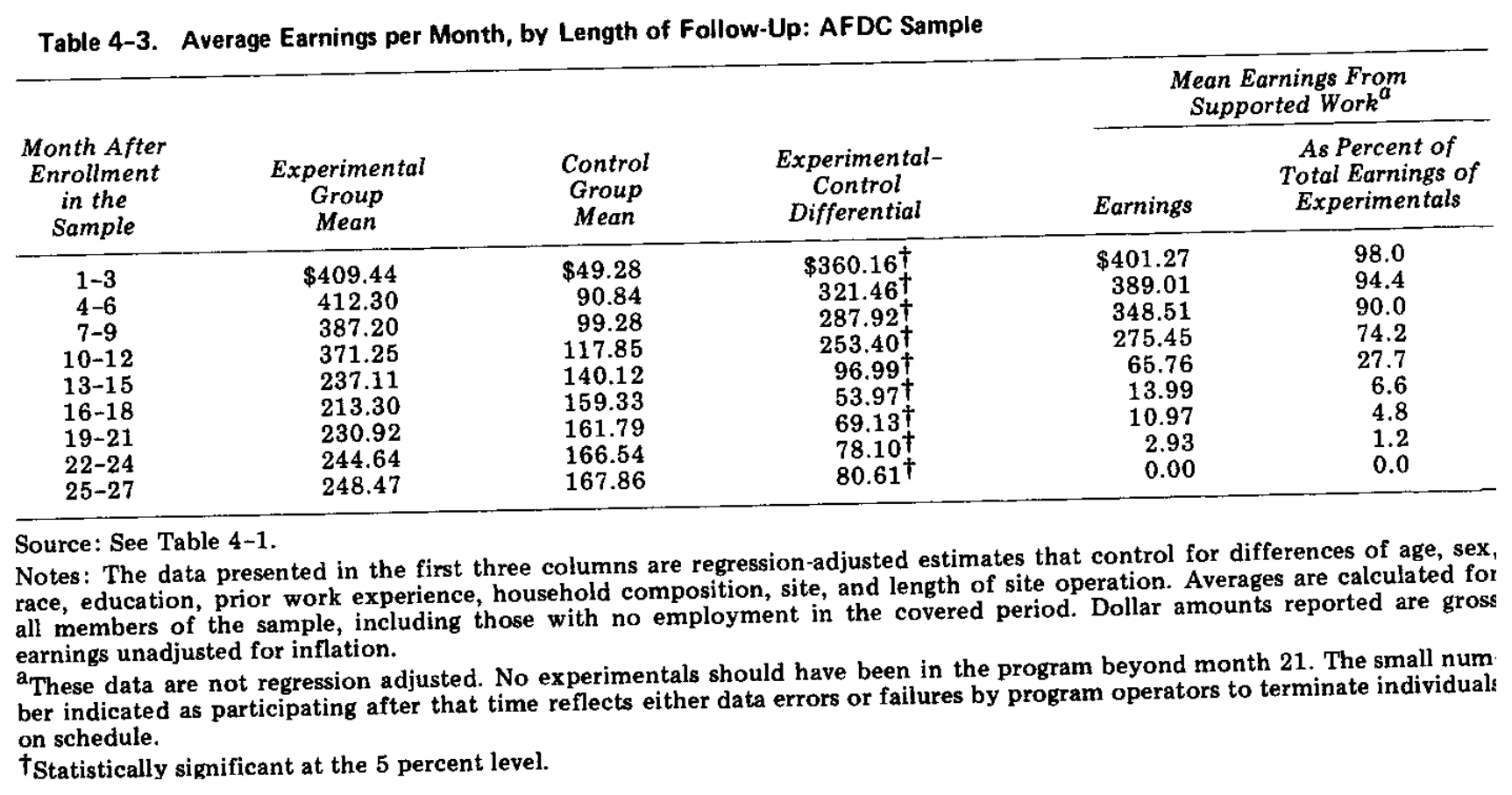
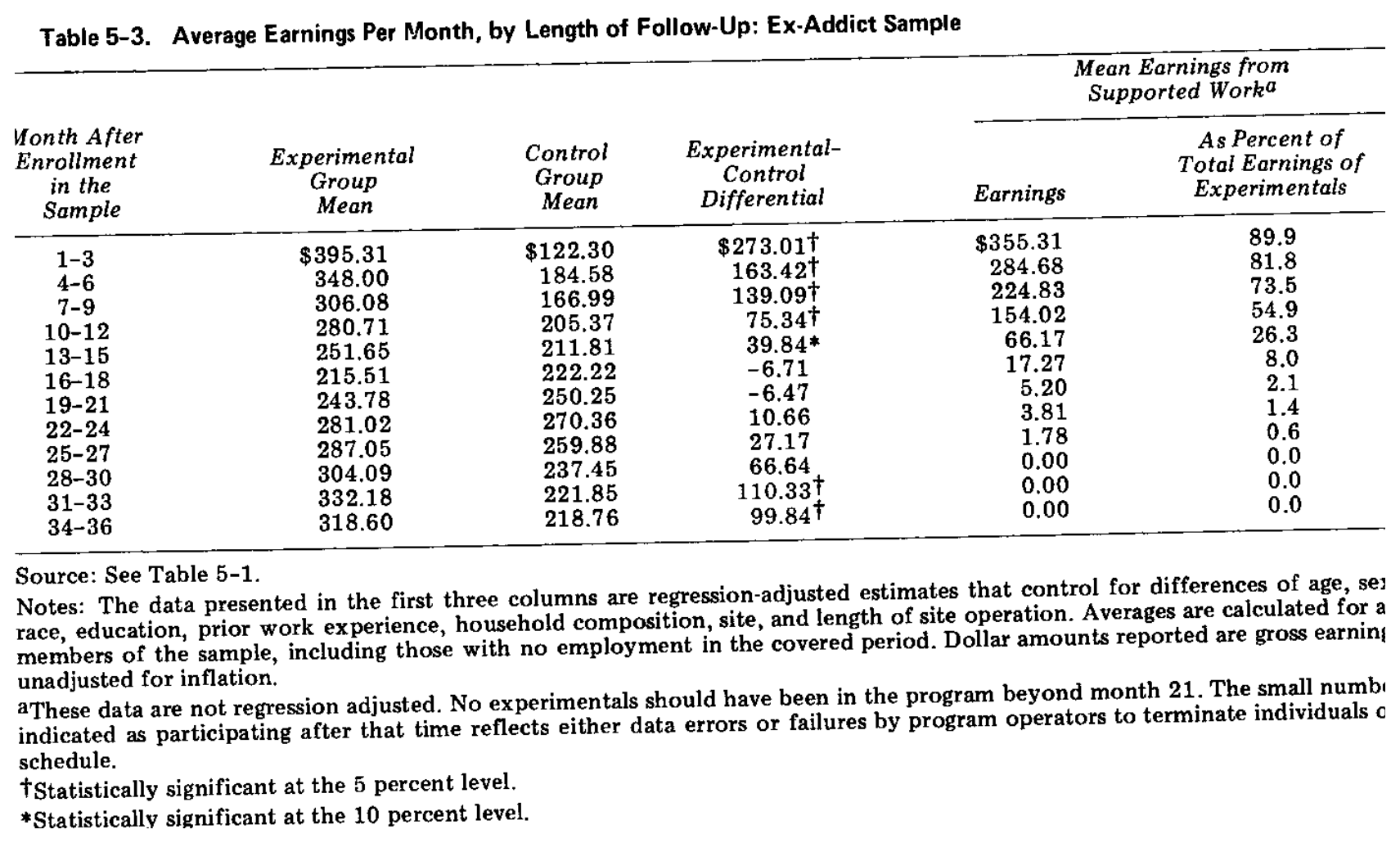
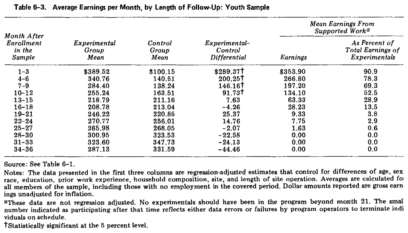
- **MDRC, *Summary and Findings of the National Supported Work Demonstration*.** Read the programme overview and research-design discussion, and examine Tables **4-3 (p. 61), 5-3 (p. 84), 6-3 (p. 106), and 7-3 (p. 124)**. Page numbers refer to the printed pages. [Report and download](https://www.mdrc.org/work/publications/summary-and-findings-national-supported-work-demonstration).
- **LaLonde (1986), “Evaluating the Econometric Evaluations of Training Programs with Experimental Data.”** Focus on the research question, experimental and comparison samples, and **Tables 3 and 5** for men. [Published paper](https://www.jstor.org/stable/1806062).
- **Dehejia and Wahba (1999), “Causal Effects in Nonexperimental Studies: Reevaluating the Evaluation of Training Programs.”** Focus on the sample, **Figures 1 and 2**, and **Table 3**. [Paper from the author's website](https://users.nber.org/~rdehejia/papers/dehejia_wahba_jasa.pdf).
The quotations used in class come from **LaLonde (1984), Chapter 2, footnote 5, printed pp. 81–82**. The working paper gives a fuller account of why his male-sample estimate differs from the report's findings. [Princeton catalogue record](https://irs.princeton.edu/publications/working-papers/evaluating-econometric-evaluations-training-programs-experimental-data).
### Textbook references
- **The Effect:** Chapter 14, *Matching*. [Online book](https://theeffectbook.net/).
- **Causal Inference: The Remix:** Chapter 5, *Unconfoundedness*, particularly matching and propensity scores. [Online book](https://mixtape.scunning.com/).
- **Mastering 'Metrics:** Chapter 2, *Regression*, for selection on observables and comparisons conditional on covariates. [Companion resources](https://www.masteringmetrics.com/online-metrics-resources/) and [Mastering Econometrics videos at Marginal Revolution University](https://learn.mru.org/courses/mastering-econometrics).
- **Mostly Harmless Econometrics, optional advanced reading:** Chapter 3, particularly regression, matching, and the propensity score. [Book contents](https://www.mostlyharmlesseconometrics.com/book-contents/).
Use the textbook references for complementary explanations of the material.
## 1. From selection bias to a credible comparison
Let $D_i=1$ indicate programme participation, and let $Y_i^1$ and $Y_i^0$ be earnings with and without treatment. The observed outcome is
$$Y_i=D_iY_i^1+\left(1-D_i\right)Y_i^0.$$
The average treatment effect on the treated is
$$\tau_{\mathrm{ATT}}=E\left[Y_i^1-Y_i^0\mid D_i=1\right].$$
We observe treated individuals' outcomes with treatment, but not what those same people would have earned without it. Recall the Week 1 decomposition:
$$
\begin{aligned}
E\left[Y_i\mid D_i=1\right]-E\left[Y_i\mid D_i=0\right]
={}&\tau_{\mathrm{ATT}}\\
&+E\left[Y_i^0\mid D_i=1\right]-E\left[Y_i^0\mid D_i=0\right].
\end{aligned}
$$
The second line is selection bias. Participants and nonparticipants may have had different earnings even without the programme.
Matching tries to make the comparison **“apples to apples”** using observed pre-treatment characteristics. Regression adjustment also addresses differences in observed characteristics, but a fitted regression can extrapolate into combinations of characteristics with little or no comparison data. Making the comparisons explicit helps us see where the evidence comes from.
## 2. Supported Work: first understand the experiment
The National Supported Work Demonstration offered temporary paid employment in a supportive, performance-oriented environment. Its policy objective was to help people with substantial employment difficulties move into regular, unsubsidised work. Its target groups included long-term recipients of Aid to Families with Dependent Children (AFDC), former drug addicts, former offenders, and young school dropouts. Eligible applicants in the experiment were randomly assigned to the treatment or control group.
Distinguish **earnings while in subsidised employment** from earnings after leaving the programme. The later outcomes tell us about the persistence of the earnings gains.
### The report's earnings tables
These tables organise outcomes by **months since enrolment**. The first three columns are regression-adjusted experimental and control means and their difference. The amounts are monthly earnings in nominal dollars. The final columns distinguish earnings received directly from Supported Work. Read the table notes as part of the evidence.
The AFDC sample supplies the discussion of women. The other three target groups were predominantly male, but **their report tables include women as well as men**. LaLonde later restricts his pooled analysis to men.
#### Table 4-3: AFDC sample
{fig-alt="MDRC Table 4-3, earnings by follow-up period for the AFDC sample."}
#### Table 5-3: ex-addict sample
{fig-alt="MDRC Table 5-3, earnings by follow-up period for the ex-addict sample."}
#### Table 6-3: youth sample
{fig-alt="MDRC Table 6-3, earnings by follow-up period for the youth sample."}
#### Table 7-3: ex-offender sample
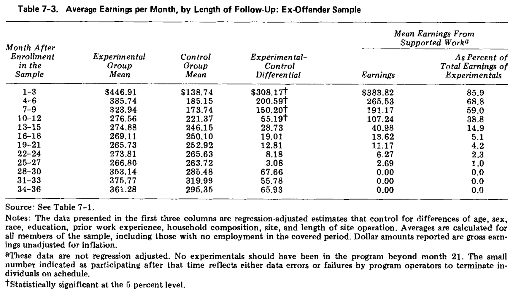{fig-alt="MDRC Table 7-3, earnings by follow-up period for the ex-offender sample."}
::: {.callout-note icon=false}
## Your turn
Explain the outcome and units, the treatment-control comparison, the magnitude and persistence of the estimated impacts, and their uncertainty. Compare the results across target groups, considering their different needs, labour-market opportunities, and follow-up periods.
:::
## 3. LaLonde: evaluating the evaluation methods
LaLonde wants to evaluate whether substituting a control group from survey or administrative data can yield the same estimate of the NSW impact as in the experiment.
The comparison groups come from the **Panel Study of Income Dynamics (PSID)** and the **Current Population Survey linked to Social Security earnings records (CPS–SSA)**. Different restrictions produce different comparison samples.
### Table 3: the data
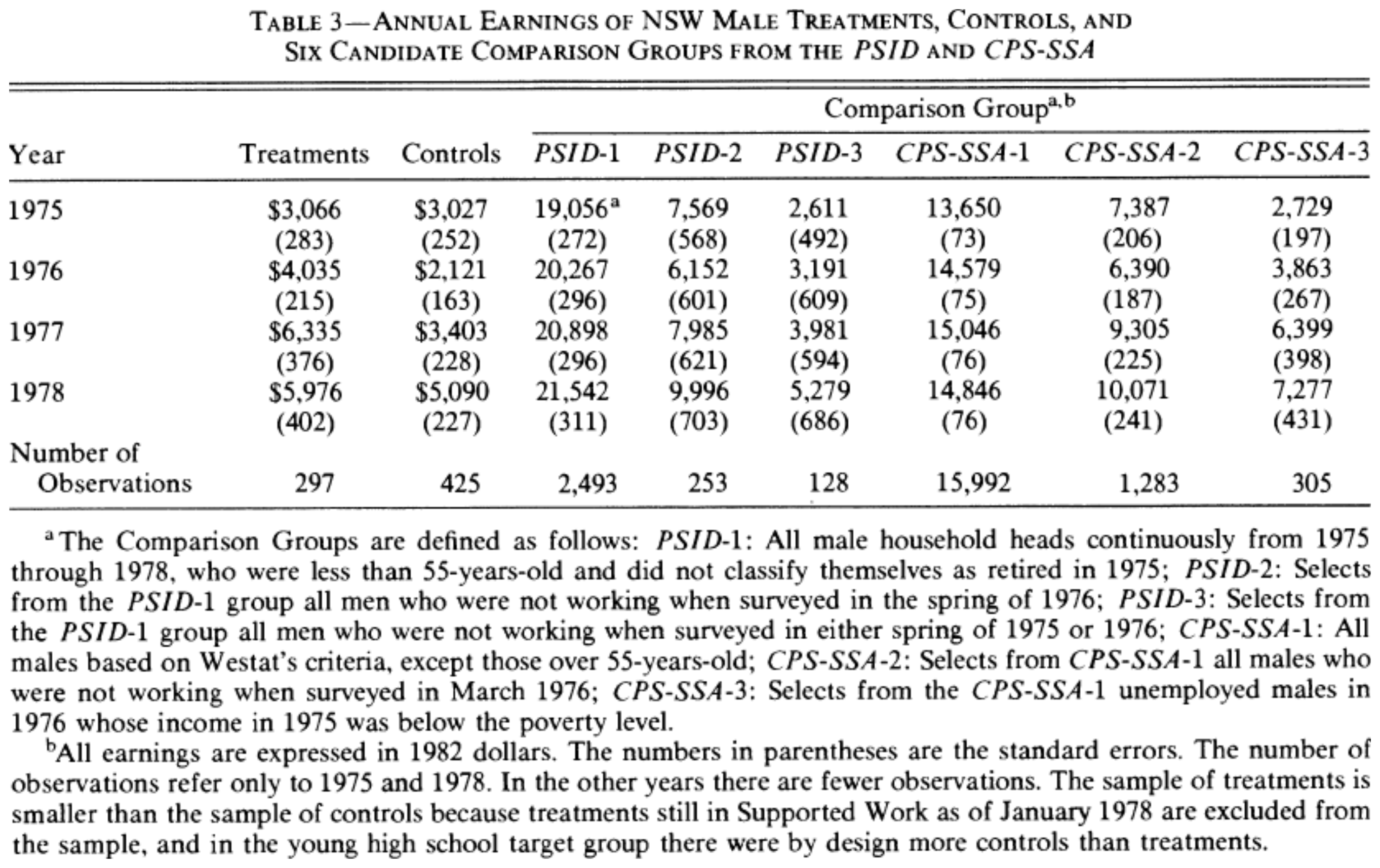{fig-alt="LaLonde Table 3: male experimental and observational samples."}
For 1978, treatment and control means are $5,976 and $5,090: a difference of **$886**, in 1982 dollars. There are **297 treated men and 425 experimental controls**. The remaining columns show how different observational comparison groups can be, including in pre-programme earnings.
### Table 5: the estimates
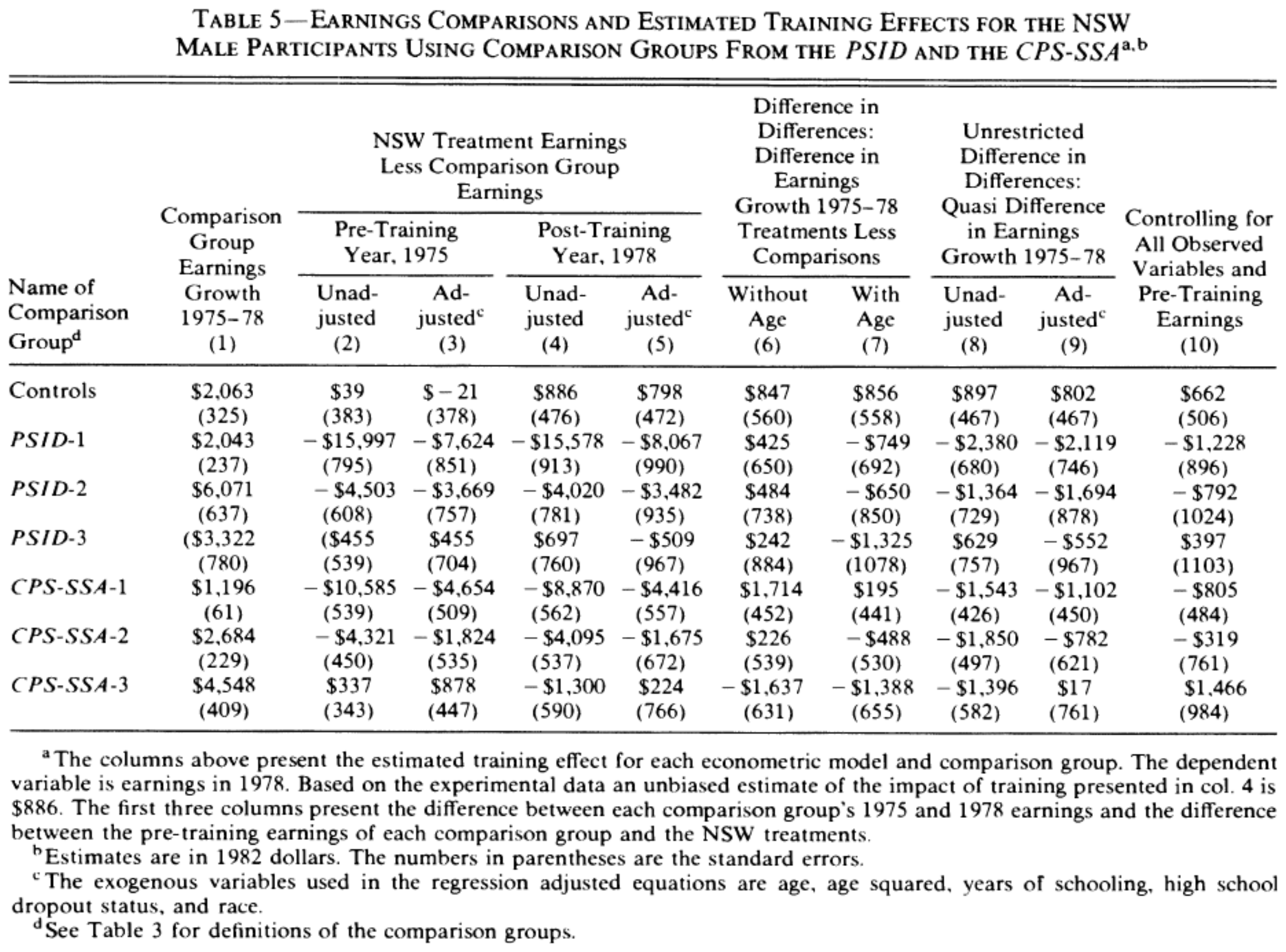{fig-alt="LaLonde Table 5: experimental and nonexperimental estimates for men."}
Focus on **column 4 (unadjusted post-training differences)** and **column 5 (regression-adjusted differences)**, comparing the controls row with the PSID and CPS–SSA rows. The standard error of the unadjusted experimental estimate is $476.
Changing the comparison group or adjustment can change the answer substantially. The question is whether the observed characteristics and adjustment adequately remove selection bias. We return to difference-in-differences later in the module.
::: {.callout-note icon=false}
## Your turn
Explain why LaLonde might have considered the samples from the PSID and CPS to be good potential sources for counterfactuals for the treated groups in the NSW experiment.
:::
### Why the experimental estimates differ
The report's target-group estimates and LaLonde's pooled male estimates differ in time units, prices, and sample construction. His annual-earnings sample has a larger share observed at the later follow-up, when the full-sample effects were larger:
> “First, the partial sample contains a much larger proportion of males who completed a 36 month interview than does the full sample. Second, the training effects for the full sample are much larger for the 36 month interview than for the 27 month interview.”
—LaLonde (1984), Chapter 2, footnote 5, pp. 81–82.
He also acknowledges that constructing the sample selected treated people with higher subsequent earnings:
> “Thus the process of selecting individuals with complete earnings in 1975 and 1978 caused us to select treatments, but not controls, with higher earnings after the 27th and 36th month interviews. Despite this potential selection bias, this paper treats the partial sample as if it was an experimental data set.”
—LaLonde (1984), Chapter 2, footnote 5, p. 82.
His Table 2.4 compares the full male sample with the annual-earnings subsample. The discussion on pp. 41–42 also recognises the problem of excluding treated people still in Supported Work in January 1978. **Random assignment in the original experiment does not guarantee that a subsequently selected sample preserves that comparison.**
## 4. Exact matching and the assumptions
Let $X_i$ collect characteristics measured before treatment, such as schooling, age, and earlier earnings. For the ATT, the central assumption is
$$Y_i^0\perp D_i\mid X_i.$$
Under **unconfoundedness**, or **selection on observables**, participation provides no further information about untreated potential earnings once we condition on $X_i$. Unobserved determinants of earnings can exist, but they must not remain associated with participation conditional on $X_i$ in a way that violates this assumption.
We also need **common support**:
$$P\left(D_i=0\mid X_i=x\right)>0
\quad\text{for }x\text{ occurring among the treated}.$$
We need to estimate what would have happened to the treated individuals if they had not received treatment. Retain the Week 1 assumptions about well-defined treatment and interference.
Under these assumptions,
$$E\left[Y_i^0\mid D_i=1,X_i=x\right]
=E\left[Y_i\mid D_i=0,X_i=x\right].$$
This step lets observed controls supply the missing counterfactual.
### Within-cell comparisons
With discrete covariates, form cells of people with exactly the same characteristics. Compare treated and control means within each cell:
$$\widehat\tau\left(x\right)=\overline Y_{D=1,X=x}-\overline Y_{D=0,X=x}.$$
For the ATT, average these differences using the treated sample's cell shares. If $N_{1x}$ is the treated count in cell $x$ and $N_1$ the total treated count,
$$\widehat\tau_{\mathrm{ATT}}=\sum_x\frac{N_{1x}}{N_1}\widehat\tau\left(x\right).$$
For example, if 75% of the treated are in a cell with an effect of $1,000 and 25% in a cell with an effect of $2,000, the ATT estimate is $1,250. Equal weighting of the two cells would answer a different question.
Exact matching becomes data intensive: ten binary covariates generate 1,024 possible cells. Continuous earnings make exact matches rarer still. Empty control cells cannot supply a counterfactual.
## 5. The propensity score
The propensity score is
$$p\left(X_i\right)=P\left(D_i=1\mid X_i\right).$$
It summarises a vector of characteristics in one number. Rosenbaum and Rubin (1983) establish the **balancing property**
$$D_i\perp X_i\mid p\left(X_i\right),$$
and show that
$$
\left(Y_i^0,Y_i^1\right)\perp D_i\mid X_i
\quad\Longrightarrow\quad
\left(Y_i^0,Y_i^1\right)\perp D_i\mid p\left(X_i\right).
$$
If conditioning on the characteristics makes treatment unconfounded, conditioning on the true score does too. For our ATT argument, the corresponding result for $Y_i^0$ is sufficient.
The score therefore lets us condition on a single number. The balancing result concerns the distribution of observed characteristics within groups with the same true score.
We will estimate the score using logit, introduced below. The theorem applies to the true score; with $\widehat p\left(X_i\right)$, examine whether the resulting adjustment actually balances covariates. Our aim is to balance the observed characteristics. Almost perfectly predicted participation may signal a lack of comparable controls.
Use characteristics measured before treatment. Subsequent employment may itself be affected by the programme.
### Estimating a probability: the LPM and logit {#lpm-and-logit}
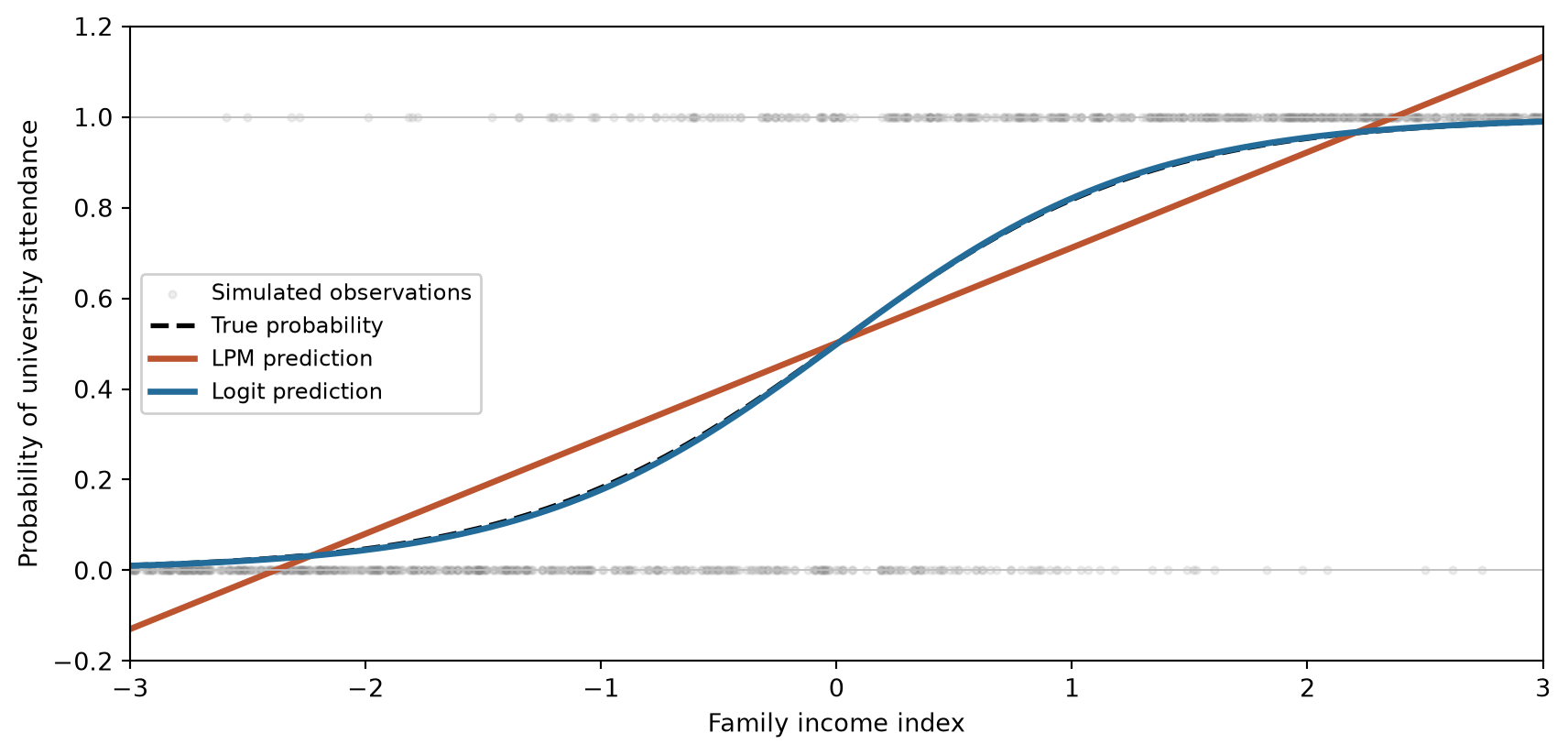
Consider a simulated example of university attendance. Let $D_i=1$ if individual $i$ attends university and $D_i=0$ otherwise. Let $X_i$ be a family-income index, with larger values representing higher incomes. Write the probability of attendance as
$$p_i=P\left(D_i=1\mid X_i\right).$$
The **linear probability model (LPM)** specifies this probability as a straight-line relationship:
$$p_i=\beta_0+\beta_1X_i.$$
We estimate its coefficients using OLS, as in Week 1. A fitted straight line can extend below zero or above one. Those predictions cannot be interpreted as probabilities.
A **logit model**, also called logistic regression, instead specifies
$$p_i=\frac{1}{1+\exp\left(-\left(\gamma_0+\gamma_1X_i\right)\right)}.$$
Here $\exp\left(z\right)=e^z$. The expression $\gamma_0+\gamma_1X_i$ is linear, but the transformation makes the probability curved and keeps it between zero and one. When the expression is zero, the probability is $0.5$; when it is $2$, the probability is about $0.88$; when it is $-2$, the probability is about $0.12$.
#### A latent-variable interpretation
We can obtain this probability model from an underlying, unobserved variable:
$$D_i^*=\gamma_0+\gamma_1X_i+\epsilon_i,$$
with the rule that $D_i=1$ when $D_i^*>0$ and $D_i=0$ otherwise. The word **latent** means unobserved. Think of $D_i^*$ as an underlying inclination to attend university. We observe whether the threshold is crossed. The disturbance $\epsilon_i$ represents other influences on the decision.
Assume that $\epsilon_i$ is independent of $X_i$ and has a **standard logistic distribution**. Its cumulative distribution function gives the probability that it is below a number $t$:
$$F\left(t\right)=P\left(\epsilon_i\leq t\right)=\frac{1}{1+\exp\left(-t\right)}.$$
Set $z_i=\gamma_0+\gamma_1X_i$. Then
$$
\begin{aligned}
P\left(D_i=1\mid X_i\right)
&=P\left(D_i^*>0\mid X_i\right)\\
&=P\left(\epsilon_i>-z_i\mid X_i\right)\\
&=1-F\left(-z_i\right)\\
&=\frac{1}{1+\exp\left(-z_i\right)}.
\end{aligned}
$$
The final equality follows from the symmetry of the logistic distribution. Its scale is set to one: multiplying the whole latent relationship by a positive constant would leave the zero-threshold decision unchanged.
#### Generate data, estimate, and plot
For the simulation, take $\gamma_0=0$, $\gamma_1=1.5$, and draw $X_i$ uniformly between $-3$ and $3$. Thus the true probability is
$$p_i=\frac{1}{1+\exp\left(-1.5X_i\right)}.$$
Conditional on income, attendance is a zero-or-one draw with probability $p_i$ of being one. We write this as $D_i\mid X_i\sim\operatorname{Bernoulli}\left(p_i\right)$. For someone with $p_i=0.8$, attendance occurs in about 80% of repeated draws. Drawing a uniform random number $U_i$ between zero and one and setting $D_i=1$ when $U_i<p_i$ would generate the same conditional distribution.
The code below uses the latent-variable construction. `rng.logistic()` draws the disturbances, and `(d_star > 0).astype(int)` converts the threshold condition to zeros and ones. We fit both models to exactly the same observations.
```{python}
#| echo: true
import numpy as np
import pandas as pd
import matplotlib.pyplot as plt
import statsmodels.formula.api as smf

rng = np.random.default_rng(5001)
n = 1000
x = rng.uniform(-3, 3, n)
epsilon = rng.logistic(loc=0, scale=1, size=n)
d_star = 1.5 * x + epsilon
d = (d_star > 0).astype(int)
simulated = pd.DataFrame({"attend": d, "income": x})

lpm = smf.ols("attend ~ income", data=simulated).fit(cov_type="HC1")
logit = smf.logit("attend ~ income", data=simulated).fit(disp=False)

grid = pd.DataFrame({"income": np.linspace(-3, 3, 400)})
grid["true_probability"] = 1 / (1 + np.exp(-1.5 * grid["income"]))
grid["lpm_prediction"] = lpm.predict(grid)
grid["logit_prediction"] = logit.predict(grid)

fig, ax = plt.subplots(figsize=(9, 4.4))
ax.scatter(simulated["income"], simulated["attend"],
           color="0.5", alpha=0.12, s=9, label="Simulated observations")
ax.plot(grid["income"], grid["true_probability"],
        color="black", linestyle="--", linewidth=2, label="True probability")
ax.plot(grid["income"], grid["lpm_prediction"],
        color="#bc542f", linewidth=2.5, label="LPM prediction")
ax.plot(grid["income"], grid["logit_prediction"],
        color="#236b99", linewidth=2.5, label="Logit prediction")
ax.axhline(0, color="0.75", linewidth=0.7)
ax.axhline(1, color="0.75", linewidth=0.7)
ax.set(xlabel="Family income index", ylabel="Probability of university attendance",
       xlim=(-3, 3), ylim=(-0.2, 1.2))
ax.legend(loc="center left", fontsize=9, framealpha=0.95)
fig.tight_layout()
plt.show()
```
In this simulation the true curve is known because we chose it. The estimated logit curve is close to it, while the LPM's straight line gives predictions below zero and above one at the ends of the observed income range. The faint points show the actual zero-or-one observations. This example illustrates the models' different shapes; real data need not follow a logistic curve.
#### What does the estimation code do?
`smf.ols()` fits the LPM. `smf.logit()` specifies the logit model, and `.fit()` estimates its coefficients by **maximum likelihood**: it chooses coefficients that make the observed pattern of attendance and non-attendance most likely under the model. The computer searches for these coefficients numerically. `disp=False` suppresses its routine progress message. The formula includes an intercept automatically.
`.predict(grid)` uses the estimated coefficients to calculate fitted probabilities at the income values in `grid`. Logit coefficients describe changes in the linear expression inside the transformation; they are not percentage-point effects as in the LPM. For propensity scores, we use the resulting predicted probabilities.
#### From this example to the propensity score
In PS1, replace attendance with `treat` and income with the listed pre-treatment characteristics. Fit the model to the 185 NSW treated men combined with **one observational comparison sample**. Here the model describes membership in the treated group within that combined sample. Refit it for the other comparison sample.
If `sample` contains that combined sample, the first PS1 model is:
```python
import statsmodels.formula.api as smf

score_model = smf.logit(
    "treat ~ age + I(age ** 2) + education + black + hispanic "
    "+ married + nodegree + I(re75 / 1000)",
    data=sample
).fit(disp=False, maxiter=200)

sample["pscore"] = score_model.predict(sample)
```
Each row now has an estimated probability between zero and one. `I(age ** 2)` includes age squared and `I(re75 / 1000)` measures earnings in thousands of dollars. `maxiter=200` allows up to 200 estimation steps. If estimation has not converged, the numerical search has not found a satisfactory solution; check the data and model before using its predictions. In Question 5, add `I(re74 / 1000)` to the formula, then estimate and predict again.
Python reference: [statsmodels Logit documentation](https://www.statsmodels.org/stable/generated/statsmodels.discrete.discrete_model.Logit.html).
## 6. Common support and Dehejia–Wahba
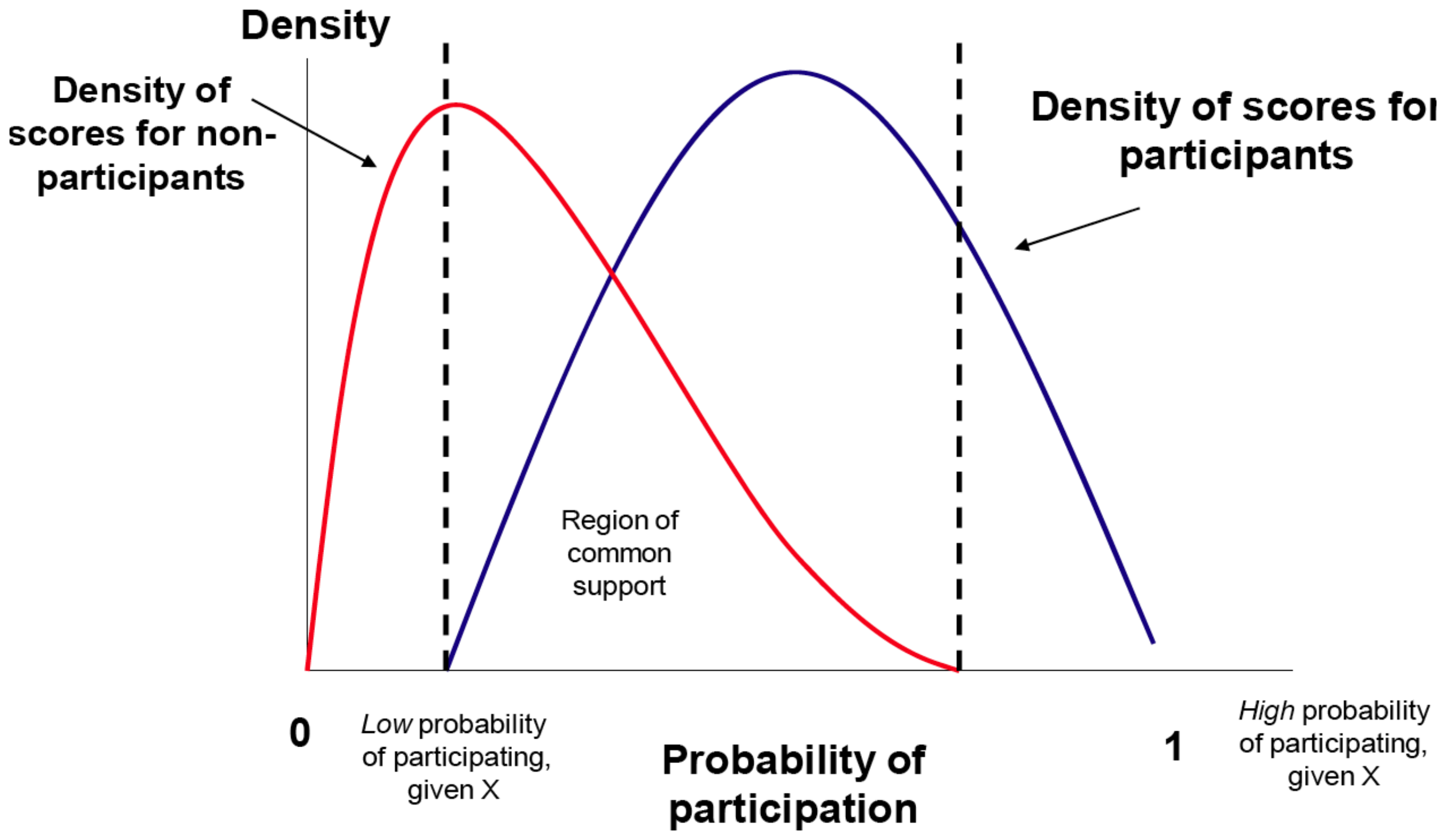{fig-alt="Illustration of common support in propensity score distributions."}
Overlap means that comparable observations exist. It can be weak even when the formal probability condition holds. If many treated observations have scores near one and few controls do, estimates may depend on a handful of controls.
Excluding controls far outside treated support can focus the comparison. Excluding **treated** observations changes the population for which the ATT is estimated. Explain how exclusions change the group whose effect is being estimated.
### Dehejia and Wahba's sample and experimental benchmark
Dehejia and Wahba use a smaller male subsample with earnings observed in 1974 and 1975: **185 treated men and 260 experimental controls**. Their unadjusted benchmark is **$1,794 (SE $633)**. It differs from $886 because it uses a different sample. **PS1 uses this 185/260 subsample throughout.** You will reproduce the DW experimental benchmark, then hold the sample fixed while comparing IPW with 1975 earnings alone and with both 1974 and 1975 earnings.
### Figure 1
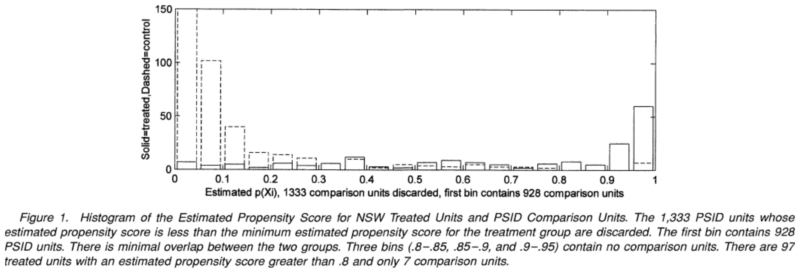{fig-alt="Dehejia and Wahba Figure 1: NSW treated and PSID comparison propensity scores."}
### Figure 2
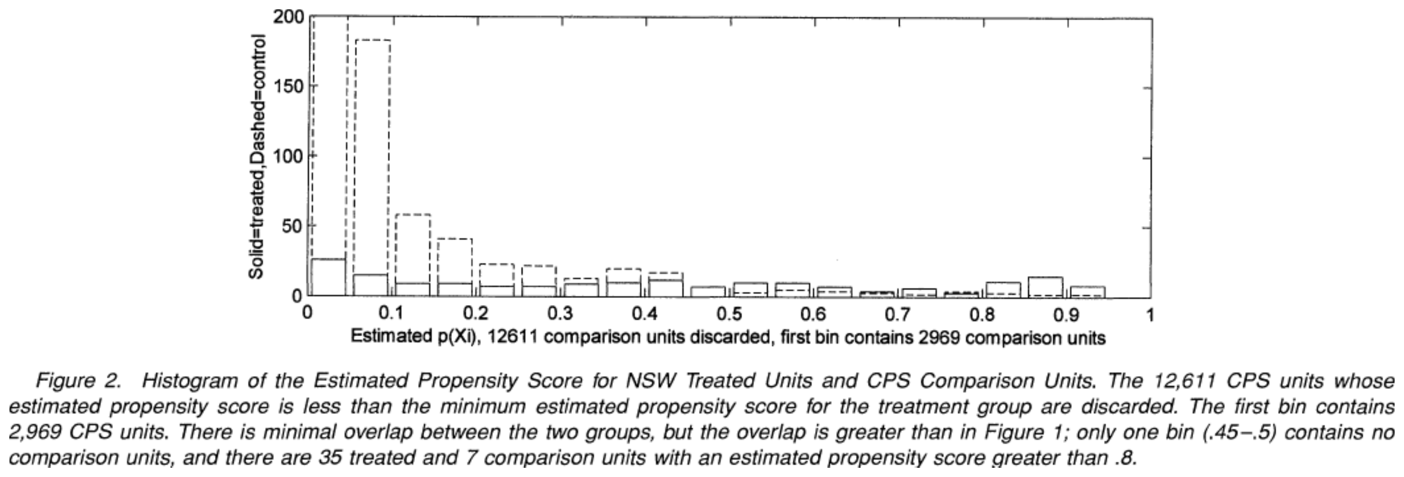{fig-alt="Dehejia and Wahba Figure 2: NSW treated and CPS comparison propensity scores."}
::: {.callout-note icon=false}
## Your turn
Identify which distribution represents the treated, where comparison observations are concentrated, and where treated people have few potential comparisons. Read the captions about discarded observations. Explain how the different sample sizes affect your interpretation of the histograms.
:::
### Table 3
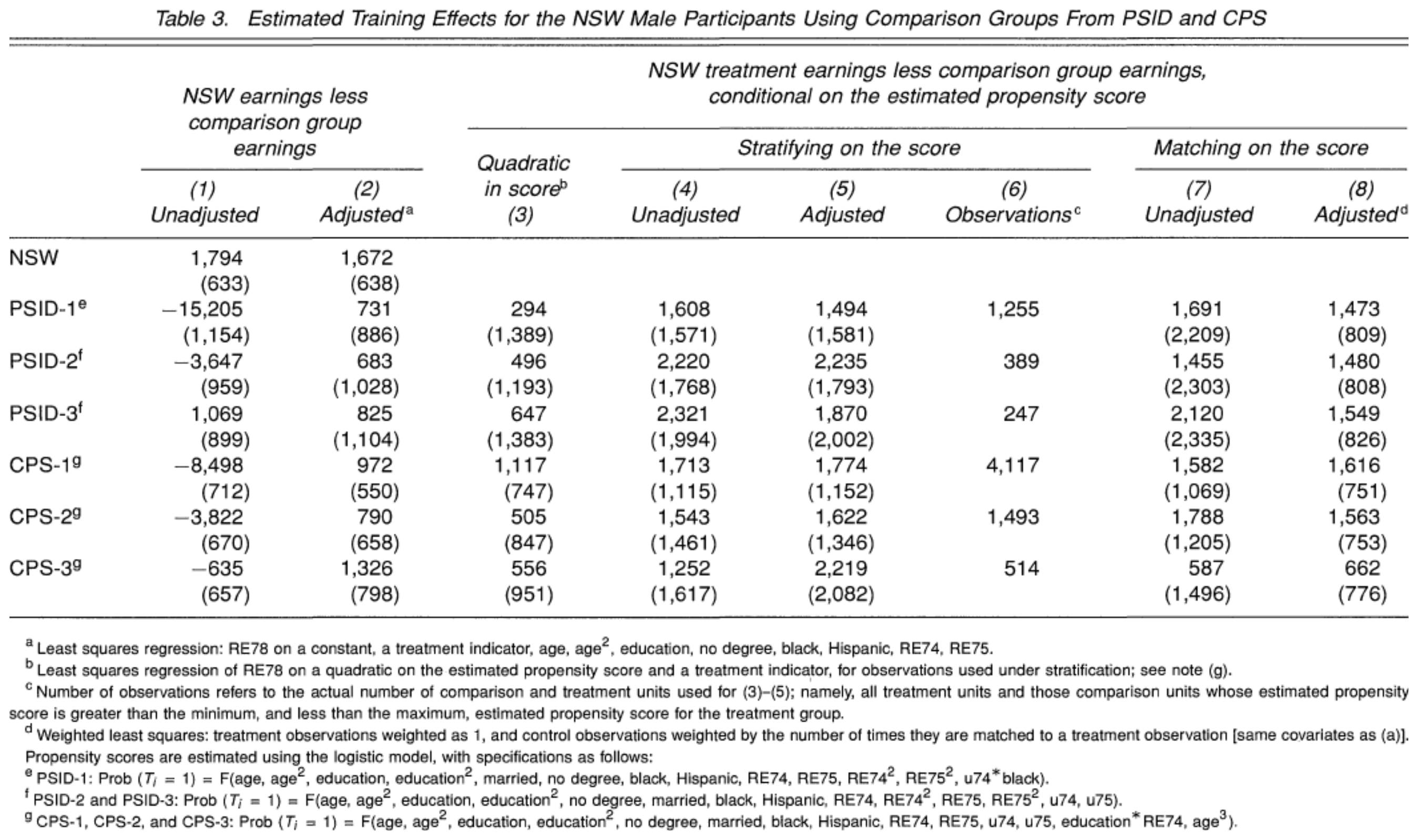{fig-alt="Dehejia and Wahba Table 3: observational estimates and NSW benchmark."}
::: {.callout-note icon=false}
## Your turn
Concentrate on the **NSW benchmark**, **column 1**, and **columns 7–8**. Explain how the estimates change and how uncertain they remain.
:::
The table's note (d) describes weights reflecting how often a control is matched. Our problem set uses the propensity-score weights introduced below.
Investigate the assignment process and data comparability. A comparison group from a different labour market, measured with different questions or lacking important work-history information, may remain problematic after adjustment. Assess the selection-on-observables assumption in the setting of each study.
### Why not simply match on the estimated score?
The propensity score's balancing property does not guarantee that matching people with similar **estimated** scores produces well-balanced samples. Similar scores can conceal substantial differences in individual characteristics. Discarding observations to improve score matches can sometimes worsen covariate balance: this is a central criticism in [King and Nielsen (2019)](https://doi.org/10.1017/pan.2019.11). Their critique concerns propensity-score matching; it does not invalidate the score's use for weighting or the population balancing result discussed above.
For our weighting exercise, **check balance in the actual covariates and inspect the weights**. Large weights can make estimates unstable.
## 7. Inverse-probability weighting for the ATT
We can use weights to construct a comparison group. **For the ATT**, keep treated observations equally weighted and reweight controls to resemble them:
$$
w_i=
\begin{cases}
1 & D_i=1,\\[4pt]
\dfrac{\widehat p\left(X_i\right)}{1-\widehat p\left(X_i\right)} & D_i=0.
\end{cases}
$$
These are **ATT weights**, often called odds weights for controls. They estimate the average treatment effect for those who received treatment by making the controls resemble the treated group.
### ATT and ATE weights
ATE weights estimate the average treatment effect for the whole population, including people who did not receive treatment. Weight each observation by the inverse of its estimated probability of receiving its observed treatment:
$$w_i^{\mathrm{ATE}}=\begin{cases}
\dfrac{1}{\widehat p\left(X_i\right)} & D_i=1,\\[6pt]
\dfrac{1}{1-\widehat p\left(X_i\right)} & D_i=0.
\end{cases}$$
Both groups are reweighted to represent the population's distribution of observed characteristics.
For NSW, our question concerns the effect on programme participants. ATT weights make the survey controls resemble those participants and address the effect we compare with the experimental benchmark. Applying ATE weights to the combined NSW-survey sample would also reweight the treated observations towards the survey respondents' characteristics. Some of those characteristics are scarcely represented among NSW participants, so a few treated observations could receive very large weights. The composition of that combined sample also depends on which survey sample we append and its size.
ATE weights are useful when the question concerns a clearly defined broader population and there is adequate overlap between its treated and control groups.
### Why these weights?
Within a covariate cell, the treated share is proportional to $p\left(x\right)$ and the control share to $1-p\left(x\right)$. To make controls represent the treated, multiply their contribution by the ratio $p\left(x\right)/\left(1-p\left(x\right)\right)$.
More formally, Bayes' rule gives
$$
\frac{f\left(x\mid D=1\right)}{f\left(x\mid D=0\right)}
=\frac{p\left(x\right)}{1-p\left(x\right)}
\frac{P\left(D=0\right)}{P\left(D=1\right)}.
$$
The last factor is constant across observations and cancels when we normalise the weighted control mean.
A control with score 0.2 receives weight $0.2/0.8=0.25$. One with score 0.8 receives $0.8/0.2=4$, sixteen times as much. At 0.95, the weight is 19. Large weights make the connection to weak common support concrete.
### From OLS to weighted least squares
In PP5000, we derived OLS using the **method of moments**. The same coefficient estimates minimise the sum of squared residuals:
$$\min_{b_0,b_1}\sum_{i=1}^n\left(Y_i-b_0-b_1D_i\right)^2.$$
Every observation receives equal weight. Here $b_0$ and $b_1$ are candidate coefficient values; the values that minimise the sum are the estimates $\widehat\beta_0$ and $\widehat\beta_1$.
Weighted least squares instead minimises
$$\min_{b_0,b_1}\sum_{i=1}^n w_i\left(Y_i-b_0-b_1D_i\right)^2.$$
An observation with a larger weight contributes more to this sum.
### IPW as a regression
Estimate
$$Y_i=\beta_0+\beta_1D_i+u_i$$
by **weighted least squares**, choosing coefficients to minimise
$$\min_{b_0,b_1}\sum_i w_i\left(Y_i-b_0-b_1D_i\right)^2.$$
Here regression calculates two group means with the desired weights. Under the identification assumptions, its treatment coefficient estimates the ATT.
Write the fitted control mean as $\mu_0=\beta_0$ and treated mean as $\mu_1=\beta_0+\beta_1$. The objective becomes
$$
\sum_{i:D_i=0}w_i\left(Y_i-\mu_0\right)^2
+\sum_{i:D_i=1}\left(Y_i-\mu_1\right)^2.
$$
Each part is minimised by its group mean:
$$
\widehat\beta_0=\frac{\sum_{i:D_i=0}w_iY_i}{\sum_{i:D_i=0}w_i},
\qquad
\widehat\beta_0+\widehat\beta_1=\frac{1}{N_1}\sum_{i:D_i=1}Y_i.
$$
Therefore,
$$
\widehat\beta_1
=\frac{1}{N_1}\sum_{i:D_i=1}Y_i
-\frac{\sum_{i:D_i=0}w_iY_i}{\sum_{i:D_i=0}w_i}.
$$
Normalising by the sum of control weights makes the second term an average. Multiplying all control weights by a common positive constant does not change this mean or treatment coefficient.
The equivalence applies to a regression with **only an intercept and treatment indicator**. Adding regressors changes the coefficient; it is no longer simply this difference in means.
### Python template
This template uses a DataFrame called <code>df</code> containing the NSW treated observations and one survey comparison group, with the columns listed below.
If `nsw_treated` and `survey_controls` are the DataFrames you imported from the two files, stack their rows as follows. Use the same variable names in both DataFrames.
~~~python
import pandas as pd

df = pd.concat([nsw_treated, survey_controls], ignore_index=True)
print(df.groupby("treat").size())
~~~
`pd.concat` stacks the observations and matches columns by name. `ignore_index=True` gives the combined data a new row index. The count checks how many treated and comparison observations it contains.
Use one analysis sample for the comparisons and report observations lost to missing values. Keep `re74` in that sample from the start so Question 5 can add it to the propensity-score model without changing the observations. The initial models below use 1975 earnings only.
~~~python
import numpy as np
import pandas as pd
import statsmodels.formula.api as smf

columns = [
    "treat", "re78", "re74", "re75", "age", "education",
    "married", "nodegree", "black", "hispanic"
]
sample = df[columns].dropna().copy()
print("Observations omitted:", len(df) - len(sample))

unadjusted = smf.ols(
    "re78 ~ treat", data=sample
).fit(cov_type="HC1", use_t=True)

adjusted = smf.ols(
    "re78 ~ treat + age + I(age ** 2) + education + married "
    "+ nodegree + black + hispanic + I(re75 / 1000)",
    data=sample
).fit(cov_type="HC1", use_t=True)

# Model treatment using pre-treatment covariates
score_model = smf.logit(
    "treat ~ age + I(age ** 2) + education + married "
    "+ nodegree + black + hispanic + I(re75 / 1000)",
    data=sample
).fit(disp=False, maxiter=200)

sample["pscore"] = score_model.predict(sample)
if not score_model.mle_retvals["converged"]:
    raise ValueError("The propensity-score model did not converge.")
if not sample["pscore"].between(0, 1, inclusive="neither").all():
    raise ValueError("Inspect the score model and common support.")

sample["att_weight"] = 1.0
controls = sample["treat"].eq(0)
sample.loc[controls, "att_weight"] = (
    sample.loc[controls, "pscore"]
    / (1 - sample.loc[controls, "pscore"])
)

# ATT-weighted regression: intercept and treatment only
weighted = smf.wls(
    "re78 ~ treat",
    data=sample,
    weights=sample["att_weight"]
).fit(cov_type="HC1", use_t=True)

print(weighted.summary())

# Check the difference-in-means interpretation
treated_mean = sample.loc[~controls, "re78"].mean()
control_mean = np.average(
    sample.loc[controls, "re78"],
    weights=sample.loc[controls, "att_weight"]
)
print("Weighted difference:", treated_mean - control_mean)
print("WLS coefficient:", weighted.params["treat"])
~~~
### Plot the propensity-score distributions
After estimating `pscore`, use the same bins and axes for both groups. `density=True` makes each histogram have total area one, allowing us to compare distribution shapes when group sizes differ.
~~~python
import matplotlib.pyplot as plt

bins = np.linspace(0, 1, 21)
fig, axes = plt.subplots(1, 2, figsize=(9, 3.5), sharex=True, sharey=True)

axes[0].hist(sample.loc[sample["treat"].eq(1), "pscore"],
             bins=bins, density=True, edgecolor="white")
axes[0].set_title("NSW treated")
axes[0].set_xlabel("Estimated propensity score")
axes[0].set_ylabel("Density")

axes[1].hist(sample.loc[sample["treat"].eq(0), "pscore"],
             bins=bins, density=True, edgecolor="white")
axes[1].set_title("Survey comparison group")
axes[1].set_xlabel("Estimated propensity score")

fig.tight_layout()
~~~
In an executable Quarto Python cell, the figure appears below the code. Compare the ranges of scores and where observations in each group are concentrated.
In PS1, add <code>I(re74 / 1000)</code> to the score model in Question 5, keeping the observations fixed. Fit the score separately for each observational comparison sample.
Pass the weights in the squared-residual criterion to <code>smf.wls</code>. See the [statsmodels WLS documentation](https://www.statsmodels.org/stable/generated/statsmodels.regression.linear_model.WLS.html).
### Standard errors
Heteroskedasticity means disturbance variance can differ across observations. Our treatment weights make the groups comparable on observed characteristics. Use **heteroskedasticity-consistent standard errors**, as in <code>.fit(cov_type="HC1", use_t=True)</code>, to allow the disturbance variance to differ across observations.
These robust WLS errors treat estimated propensity-score weights as fixed. A full calculation of uncertainty also accounts for estimating the propensity score.
## 8. Diagnose the comparison
Inspect score distributions and the largest control weights before interpreting the coefficient. If Python reports a warning or cannot estimate the model, check your data import and regression code. You can ask Claude to explain the message and help diagnose the problem. Make sure you understand any suggested changes before using them.
Compare **unweighted and weighted covariate balance**. The weighted control mean of a covariate is
$$\overline X_{0,w}=\frac{\sum_{i:D_i=0}w_iX_i}{\sum_{i:D_i=0}w_i}.$$
A standardised mean difference helps compare covariates in different units. One convention is
$$
\mathrm{SMD}_{w}
=\frac{\overline X_1-\overline X_{0,w}}
{\sqrt{\left(s_1^2+s_0^2\right)/2}},
$$
where $s_1^2$ and $s_0^2$ are the **unweighted** within-group variances. Keep the denominator fixed before and after weighting, so changes reflect improved mean balance.
Here `sample` continues to contain both groups. `treated` and `control_group` are the two subsets used to calculate balance.
~~~python
covariates = [
    "age", "education", "married", "nodegree",
    "black", "hispanic", "re75"
]
treated = sample.loc[sample["treat"].eq(1)]
control_group = sample.loc[sample["treat"].eq(0)]
rows = []

for variable in covariates:
    mean1 = treated[variable].mean()
    mean0 = control_group[variable].mean()
    mean0w = np.average(
        control_group[variable], weights=control_group["att_weight"]
    )
    scale = np.sqrt(
        (treated[variable].var() + control_group[variable].var()) / 2
    )
    rows.append({
        "Covariate": variable,
        "Treated mean": mean1,
        "Control mean": mean0,
        "Weighted control mean": mean0w,
        "SMD before": (mean1 - mean0) / scale if scale > 0 else np.nan,
        "SMD after": (mean1 - mean0w) / scale if scale > 0 else np.nan
    })

balance = pd.DataFrame(rows).set_index("Covariate")
print(balance.round(3))
print(control_group["att_weight"].describe(
    percentiles=[0.5, 0.9, 0.95, 0.99]
))
~~~
Mean balance can conceal distributional differences. Inspect earlier earnings and the frequency of zero earnings. Poor balance means the adjustment has not achieved its observed-data objective; good balance still leaves unconfoundedness to be defended.
## 9. Preparing for Problem Set 1
Compare OLS and ATT weighting with the experimental benchmark using **two observational comparison samples**. Explain why the estimates differ.
Your Quarto document should combine code, labelled output, and prose explaining the comparison group, sample, units, assumptions, overlap, balance, and results. The [assignment](../exercises/02-matching.qmd) specifies the data and required tasks.
## References
- Manpower Demonstration Research Corporation (1980). *Summary and Findings of the National Supported Work Demonstration*. Cambridge, MA: Ballinger. [Report](https://www.mdrc.org/work/publications/summary-and-findings-national-supported-work-demonstration).
- LaLonde, Robert J. (1984). *Evaluating the Econometric Evaluations of Training Programs with Experimental Data*. Industrial Relations Section Working Paper 183, Princeton University. [Record](https://irs.princeton.edu/publications/working-papers/evaluating-econometric-evaluations-training-programs-experimental-data).
- LaLonde, Robert J. (1986). “Evaluating the Econometric Evaluations of Training Programs with Experimental Data.” *American Economic Review* 76(4): 604–620. [Paper](https://www.jstor.org/stable/1806062).
- Rosenbaum, Paul R., and Donald B. Rubin (1983). “The Central Role of the Propensity Score in Observational Studies for Causal Effects.” *Biometrika* 70(1): 41–55. [DOI](https://doi.org/10.1093/biomet/70.1.41).
- Dehejia, Rajeev H., and Sadek Wahba (1999). “Causal Effects in Nonexperimental Studies: Reevaluating the Evaluation of Training Programs.” *Journal of the American Statistical Association* 94(448): 1053–1062. [Paper](https://users.nber.org/~rdehejia/papers/dehejia_wahba_jasa.pdf).
- King, Gary, and Richard Nielsen (2019). “Why Propensity Scores Should Not Be Used for Matching.” *Political Analysis* 27(4): 435–454. [DOI](https://doi.org/10.1017/pan.2019.11).