Matching

PP5001 · Week 2

Professor David A. Jaeger

From Random Assignment to Selection on Observables

Last week, random assignment gave us a credible comparison group. What can we do when participation is not randomly assigned?

E\left[Y_i\mid D_i=1\right]-E\left[Y_i\mid D_i=0\right] =\underbrace{E\left[Y_i^1-Y_i^0\mid D_i=1\right]}_{\text{ATT}} +\underbrace{E\left[Y_i^0\mid D_i=1\right]-E\left[Y_i^0\mid D_i=0\right]}_{\text{selection bias}}.

Matching aims to make an “apples to apples” comparison using observed characteristics. Whether it removes selection bias depends on what we observe and how participation is determined.

The Supported Work Experiment

For discussion

Impacts for Women: Table 4-3

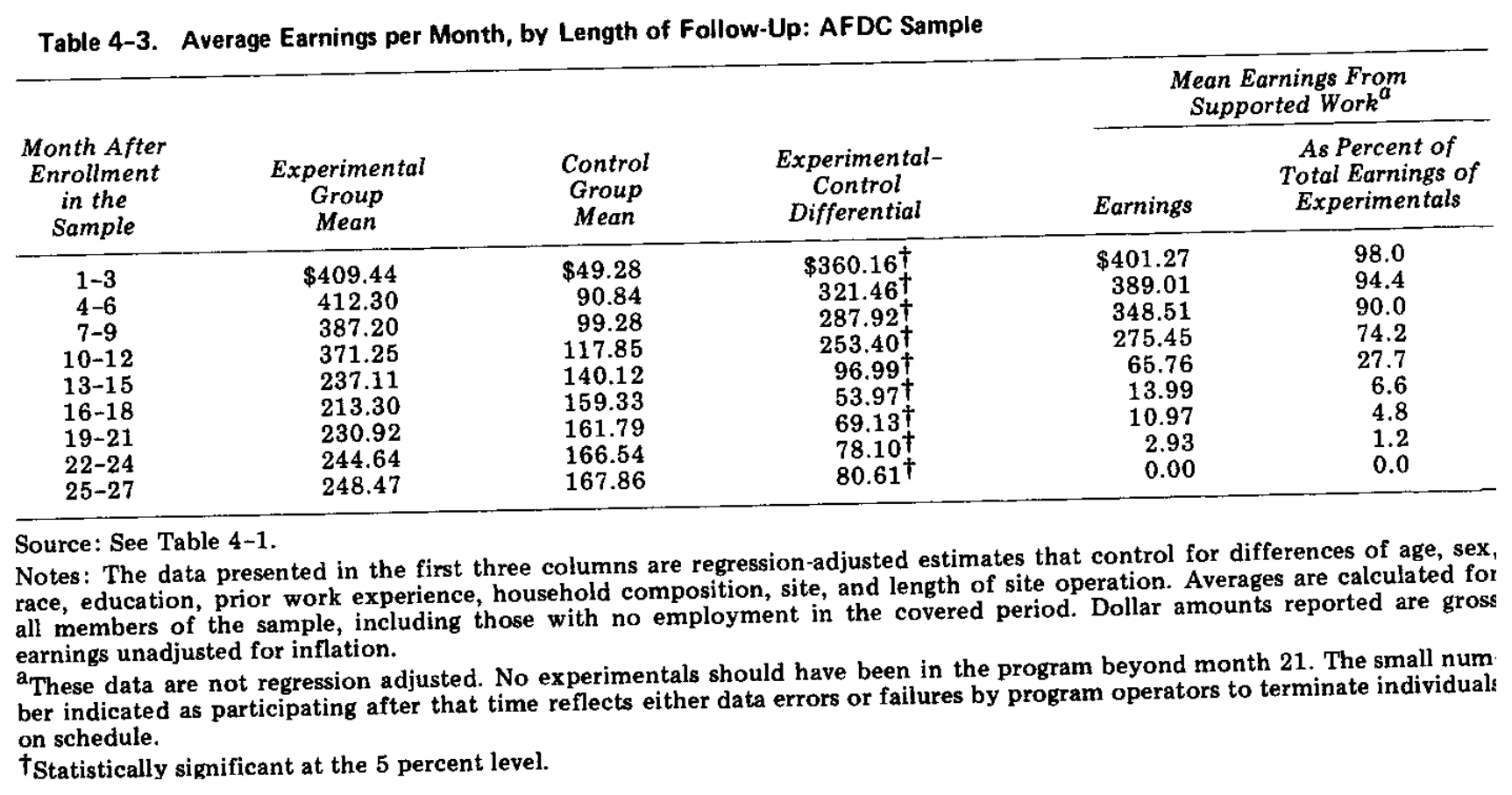
Ex-Addict Sample: Table 5-3

The report’s non-AFDC target groups include women as well as men. Explain this distinction verbally before discussing the tables; LaLonde subsequently restricts his pooled analysis to men.

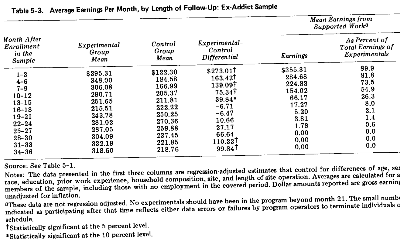
Youth Sample: Table 6-3

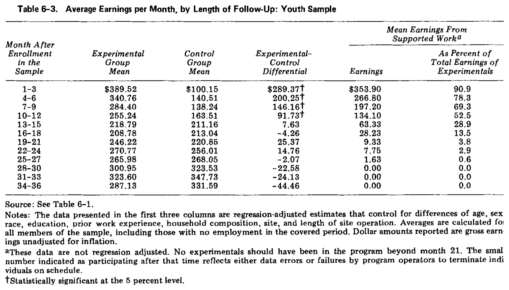
Ex-Offender Sample: Table 7-3

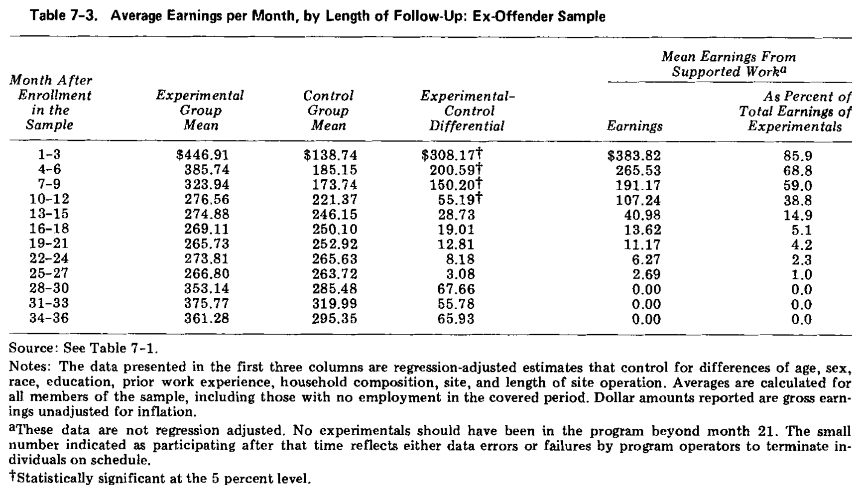
Comparing the Results

For discussion

What Is LaLonde Doing?

For discussion

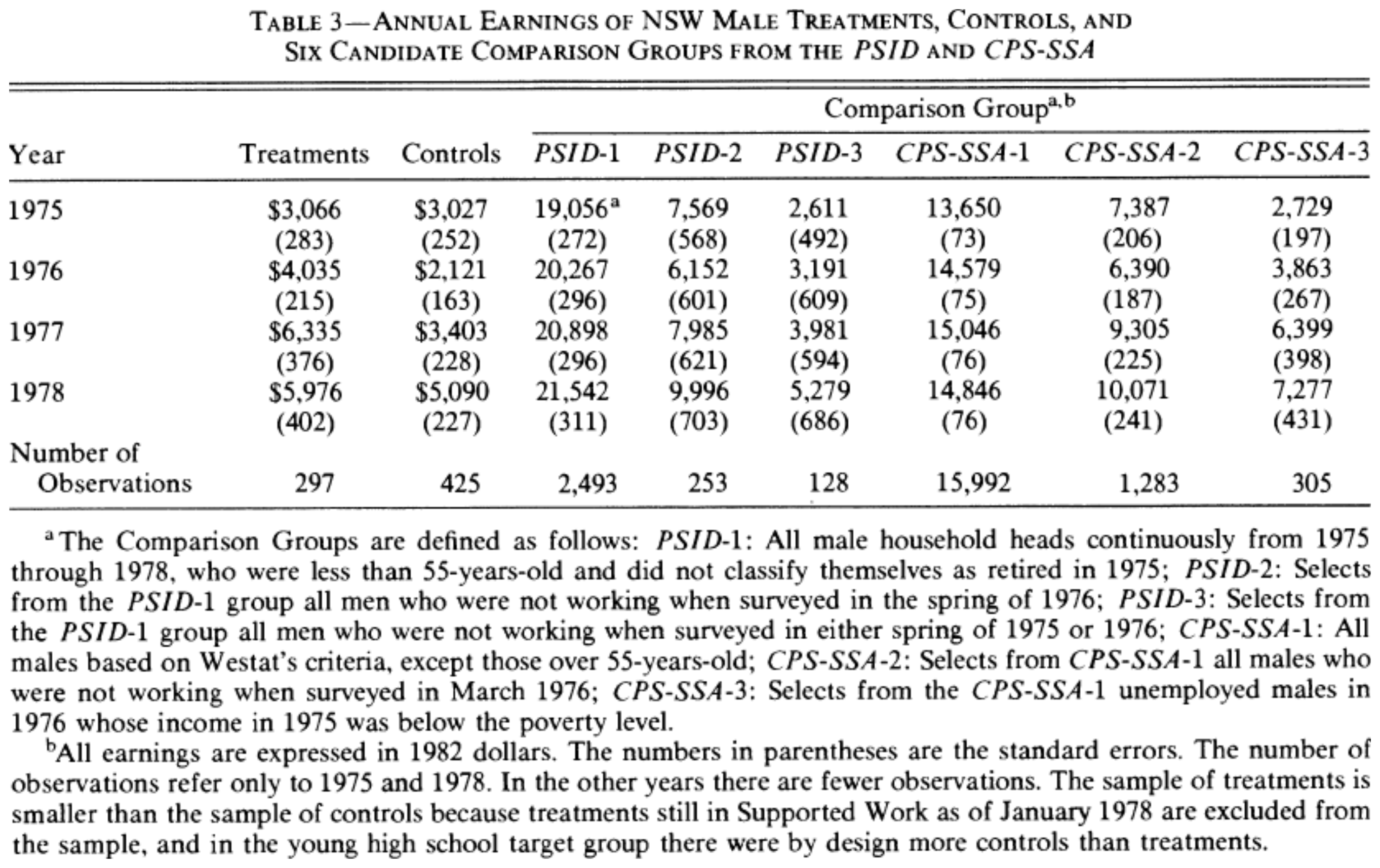
Data

For discussion

LaLonde: Table 3

LaLonde: Table 5

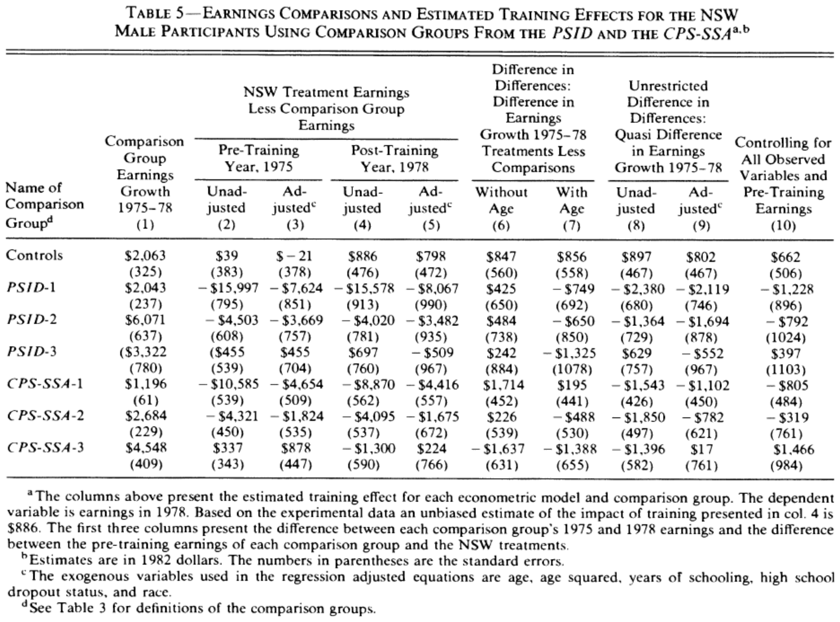
Why Do the Experimental Estimates Differ?

For discussion

LaLonde on Follow-up Timing

“First, the partial sample contains a much larger proportion of males who completed a 36 month interview than does the full sample. Second, the training effects for the full sample are much larger for the 36 month interview than for the 27 month interview.”

LaLonde (1984), Chapter 2, footnote 5, pp. 81–82.

LaLonde on Sample Selection

“Thus the process of selecting individuals with complete earnings in 1975 and 1978 caused us to select treatments, but not controls, with higher earnings after the 27th and 36th month interviews. Despite this potential selection bias, this paper treats the partial sample as if it was an experimental data set.”

LaLonde (1984), Chapter 2, footnote 5, p. 82.

What Makes a Comparison “Apples to Apples”?

People who enter a training programme may differ from other workers in their schooling, work history, and previous earnings.

Let X_i collect pre-treatment characteristics. We want nonparticipants with characteristics comparable to those of the participants.

This is more demanding than finding people with the same average age. We need comparable combinations of characteristics—and an argument that the remaining differences do not determine untreated outcomes.

Matching cannot repair an important confounder that we have not measured.

The Assumptions for the ATT

Selection on observables (unconfoundedness):

Y_i^0\perp D_i\mid X_i.

Given X_i, treatment status provides no further information about the outcome that would occur without treatment.

Common support: for every combination of X_i among treated individuals, there must be potential controls:

P\left(D_i=0\mid X_i\right)>0.

We also retain the consistency and no-interference assumptions discussed in Week 1. Their credibility depends on the study design and setting.

Exact Matching

The simplest form of matching compares individuals with the exact same set of observable characteristics.

Under unconfoundedness, compare average outcomes within the cells defined by the X’s:

\widehat\tau\left(x\right)=\overline Y_{D=1,X=x}-\overline Y_{D=0,X=x}.

For example, compare participants and nonparticipants with the same schooling and pre-programme employment history.

The control mean in each cell supplies the missing untreated outcome for treated individuals in that cell.

Averaging the Comparisons

For the ATT, average the within-cell differences using the distribution of characteristics among treated individuals.

Cell	Share of treated	Treated mean	Control mean	Difference
X=a	0.75	6,000	5,000	1,000
X=b	0.25	8,000	6,000	2,000

\widehat\tau_{\mathrm{ATT}}=0.75\left(1{,}000\right)+0.25\left(2{,}000\right)=1{,}250.

This illustrative calculation weights each treated person’s comparison equally. Using a different population’s cell shares would target a different average effect.

Why Exact Matching Becomes Difficult

Exact matching is extremely data intensive.

• With several characteristics, the number of combinations grows quickly: ten binary characteristics produce 2^{10}=1{,}024 cells.
• With continuous covariates, such as previous earnings, exact matches may be rare.
• Some cells contain treated individuals but no controls.

Adding relevant characteristics can make the assumption more plausible while making comparable observations harder to find.

The Propensity Score

The propensity score is the probability of receiving treatment conditional on the observed characteristics:

p\left(X_i\right)=P\left(D_i=1\mid X_i\right).

X_i is a vector; p\left(X_i\right) is a single number.

We will use logit to estimate this probability from pre-treatment characteristics.

The purpose is to make the groups comparable on observed characteristics.

Estimating a Probability: LPM and Logit

Let D_i indicate university attendance and X_i measure family income.

\begin{aligned} \text{LPM:}\quad p_i&=\beta_0+\beta_1X_i,\\[4pt] \text{Logit:}\quad p_i&=\frac{1}{1+\exp\left(-\left(\gamma_0+\gamma_1X_i\right)\right)}. \end{aligned}

Logit transforms the linear expression into a probability between zero and one.

Latent-variable interpretation: D_i^*=\gamma_0+\gamma_1X_i+\epsilon_i; attendance occurs when D_i^*>0.

If \epsilon_i is independent of X_i and standard logistic, this produces the logit probability above.

LPM and Logit: A Simulated Comparison

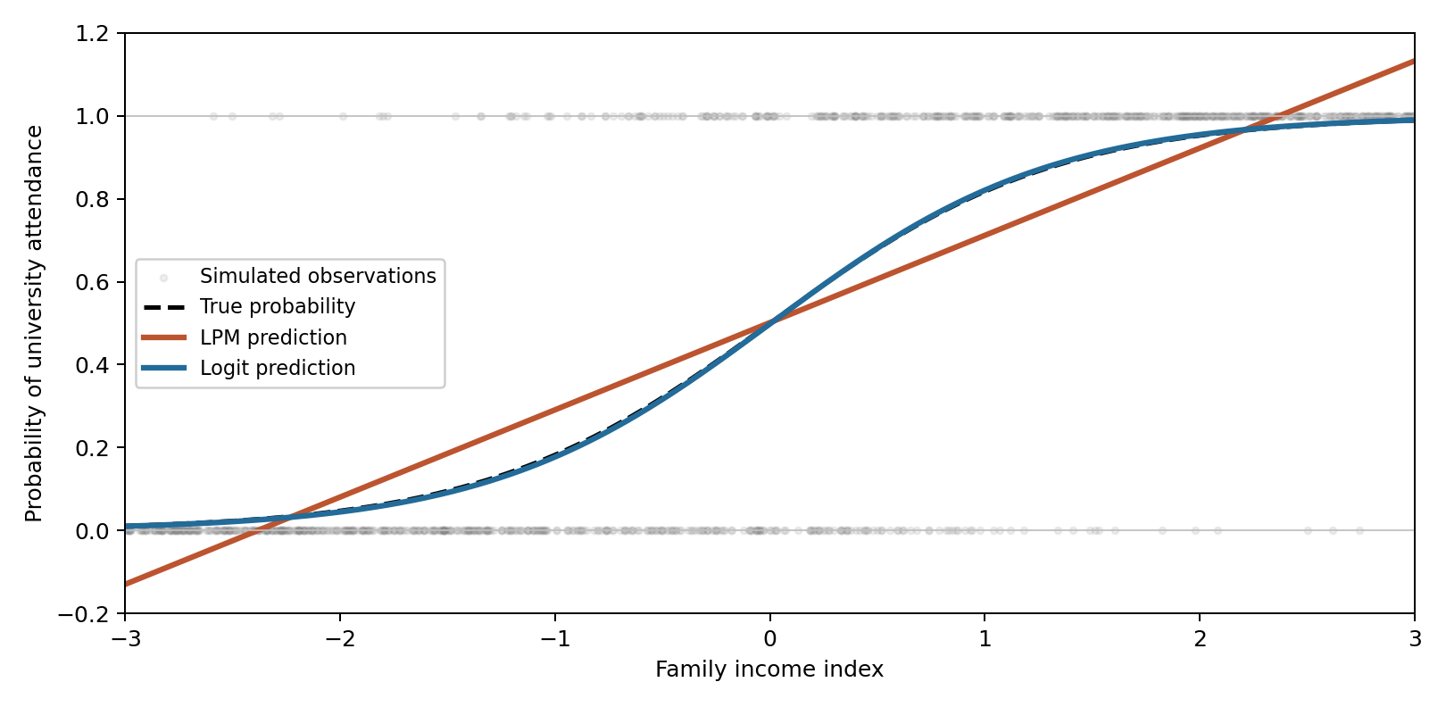
Fit with smf.ols() or smf.logit(), then use .predict() to obtain fitted probabilities. The notes give the full simulation and estimation code.

Rosenbaum and Rubin: Dimension Reduction

Rosenbaum and Rubin (1983) show that

\left(Y_i^0,Y_i^1\right)\perp D_i\mid X_i \quad\Longrightarrow\quad \left(Y_i^0,Y_i^1\right)\perp D_i\mid p\left(X_i\right).

The key balancing property is

D_i\perp X_i\mid p\left(X_i\right).

If conditioning on X_i makes assignment unconfounded, conditioning on the true propensity score does too. This reduces the dimension of the adjustment under the original assumption.

The True Score and the Estimated Score

For the true score, balancing is a theorem. For an estimated score, balance is something we must check.

The balancing result concerns the distribution of characteristics in the treated and control groups conditional on the score.

After matching or weighting, examine whether the observed characteristics are actually balanced.

Common Support

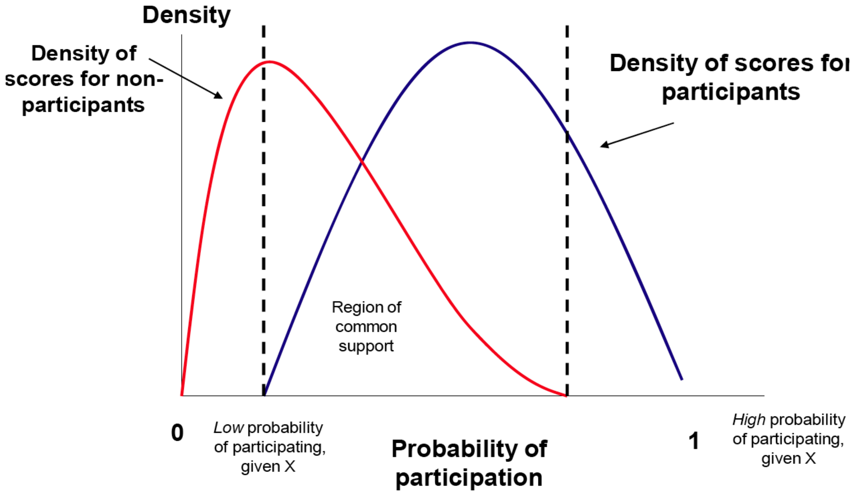
When Comparable Controls Are Scarce

For the ATT, we need controls wherever the treated observations are.

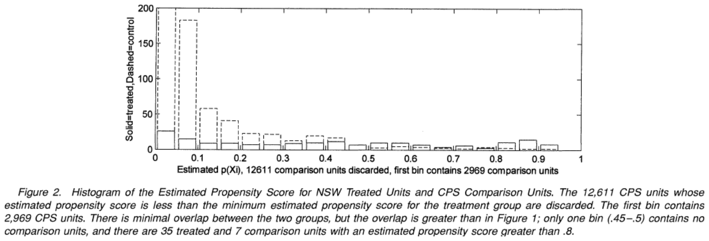
When p\left(X_i\right) is close to one, there may be many treated individuals and very few comparable controls. The estimate can depend heavily on those few controls.

Excluding treated observations without support changes the population whose effect we estimate. The estimate then applies to the retained group.

Credible comparisons require observations with comparable characteristics.

Dehejia and Wahba: The Sample

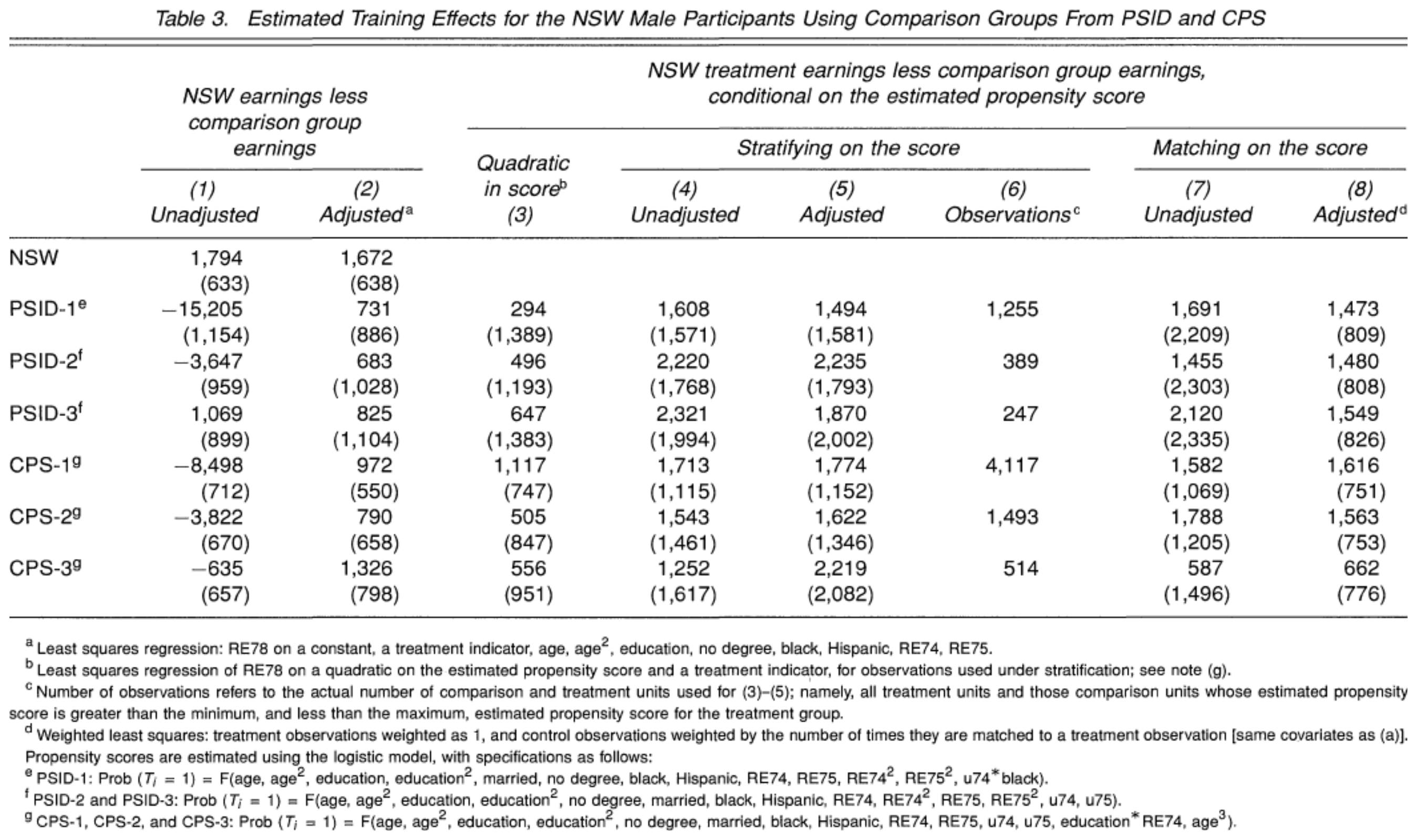
Dehejia and Wahba (1999) reanalyse the male sample.

They use the subsample with 1974 earnings available: 185 treated men and 260 experimental controls, compared with LaLonde’s 297 and 425. This gives two years of pre-programme earnings, 1974 and 1975.

Their unadjusted experimental benchmark is $1,794, rather than LaLonde’s $886.

PS1 uses this subsample throughout: reproduce its experimental benchmark, then compare IPW using one versus two years of pre-treatment earnings.

Figure 1

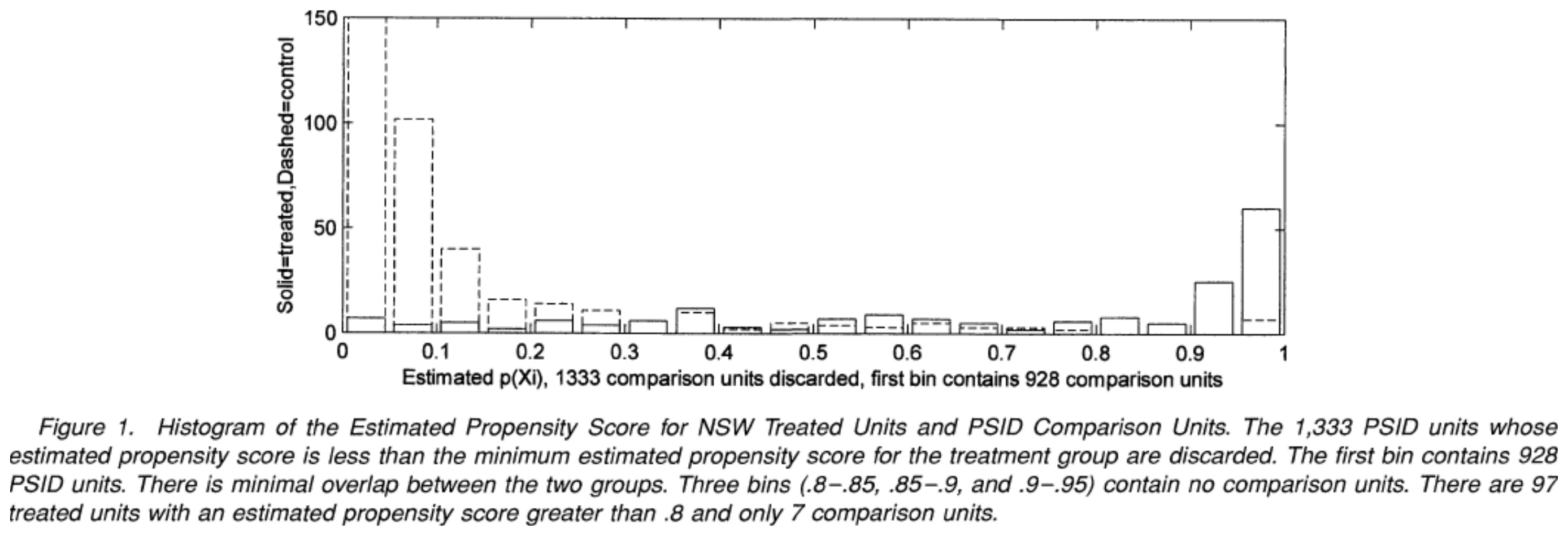
Figure 2

Dehejia and Wahba: Table 3

What Should We Learn from the Comparison?

Propensity-score adjustment can substantially change the estimates. Assess unconfoundedness using the assignment process and available characteristics in each application.

The data comparability lesson from your reading matters:

• Do the groups face comparable labour markets?
• Are outcomes and covariates measured in the same way?
• Do we observe the characteristics that jointly predict participation and outcomes?

Good balance on measured characteristics is useful evidence about the adjustment. It cannot establish balance on unmeasured confounders.

From Matching to Weighting

Instead of selecting particular controls as matches, we can give controls different weights.

For the ATT, retain the treated sample and reweight the controls to resemble it on observed characteristics.

Controls whose characteristics make treatment more likely receive greater weight. Controls who look unlike the treated receive less weight.

This is propensity-score weighting, using ATT weights.

ATT Weights

w_i= \begin{cases} 1 & \text{if }D_i=1,\\[4pt] \dfrac{\widehat p\left(X_i\right)}{1-\widehat p\left(X_i\right)} & \text{if }D_i=0. \end{cases}

Among people with characteristics X_i, the treated-to-control ratio is proportional to p\left(X_i\right)/\left(1-p\left(X_i\right)\right).

Weighting controls by these odds of treatment makes their covariate distribution resemble the treated distribution, under the population relationship and with a correctly estimated score.

For the ATE, weights are 1/\widehat p\left(X_i\right) for treated observations and 1/\left(1-\widehat p\left(X_i\right)\right) for controls. Both groups represent the whole population.

For NSW, we use the ATT to estimate the effect on participants.

What Do the Weights Mean?

Control’s estimated score	ATT weight
0.20	0.25
0.50	1.00
0.80	4.00
0.95	19.00

A control with a score of 0.80 receives sixteen times the weight of one with a score of 0.20.

The last row links weighting directly to common support: a few controls can dominate the weighted comparison.

IPW Regression: Weighted Least Squares

In PP5000, we derived OLS using the method of moments. The same estimates minimise the sum of squared residuals:

\min_{b_0,b_1}\sum_i\left(Y_i-b_0-b_1D_i\right)^2.

Every observation receives equal weight. Weighted least squares minimises

\min_{b_0,b_1}\sum_i w_i\left(Y_i-b_0-b_1D_i\right)^2.

An observation with a larger weight contributes more to the sum. The minimising values are \widehat\beta_0 and \widehat\beta_1.

For IPW, use the ATT weights to make the controls resemble the treated group.

The Coefficient Is a Difference in Means

With only an intercept and treatment indicator,

\widehat\beta_1 =\underbrace{\frac{1}{N_1}\sum_{i:D_i=1}Y_i}_{\text{treated mean}} -\underbrace{ \frac{\sum_{i:D_i=0}w_iY_i} {\sum_{i:D_i=0}w_i} }_{\text{weighted control mean}}.

The intercept estimates the weighted control mean; intercept plus treatment coefficient estimates the treated mean.

Dividing by the sum of control weights makes the second term a weighted average. Under our assumptions, it estimates the treated group’s mean outcome without treatment.

Check the Comparison Before Interpreting the Effect

1. Plot the propensity scores for both groups: is there common support?
2. Inspect control weights: does the comparison depend on a few people?
3. Compare covariate balance before and after weighting.
4. Report the estimated effect, its units, and uncertainty.

Use heteroskedasticity-consistent standard errors for the outcome regression. Ordinary WLS standard errors are inappropriate for these treatment weights.

Robust WLS errors treat estimated weights as fixed; fuller inference must also account for estimating the propensity score.

Problem Set 1

The Week 2 practice will be Problem Set 1.

Compare the experimental benchmark with estimates using two nonexperimental comparison samples:

• Unadjusted and covariate-adjusted OLS.
• ATT weighting via WLS: 1975 earnings alone, then add 1974 earnings.
• Common support, weights, balance, and interpretation.

Submit your Quarto source and rendered PDF, combining Python, results, and explanation. Due Friday 2 October, 12 noon.

Problem Set 1: instructions and Quarto answer template

References

• MDRC (1980). Summary and Findings of the National Supported Work Demonstration. Tables 4-3, 5-3, 6-3, 7-3.

• LaLonde, R. J. (1984). Evaluating the Econometric Evaluations of Training Programs with Experimental Data. Princeton IRS Working Paper 183, Chapter 2.

• LaLonde, R. J. (1986). “Evaluating the Econometric Evaluations of Training Programs with Experimental Data.” AER 76(4): 604–620.

• Rosenbaum, P. R., and D. B. Rubin (1983). “The Central Role of the Propensity Score in Observational Studies for Causal Effects.” Biometrika 70(1): 41–55.

• Dehejia, R. H., and S. Wahba (1999). “Causal Effects in Nonexperimental Studies: Reevaluating the Evaluation of Training Programs.” JASA 94(448): 1053–1062.

• King, G., and R. Nielsen (2019). “Why Propensity Scores Should Not Be Used for Matching.” Political Analysis 27(4): 435–454. DOI.

Textbook readings and links: Week 2 notes.