Two-Way Fixed Effects and Event Studies
PP5001 · Week 9 · Martinmas 2026
Professor David A. Jaeger
Recall: The Two-Period DiD
Let T_i indicate membership in the treatment group and Post_t indicate the post-treatment period.
Y_{it}=\alpha+\gamma T_i+\tau Post_t
+\delta\left(T_i\cdot Post_t\right)+u_{it}.
- \gamma allows the groups to have different initial levels.
- \tau captures their common change over time.
- \delta measures the additional change in the treatment group.
A causal interpretation requires parallel trends in untreated potential outcomes.
Multiple Units and Multiple Periods
Suppose we observe the same units over several periods. For now, treated units share one treatment date and the control units remain untreated.
Y_{it}=\alpha_i+\lambda_t+\delta D_{it}+u_{it},
\qquad D_{it}=T_i\cdot Post_t.
- \alpha_i: a separate intercept for each unit.
- \lambda_t: a separate effect for each calendar period.
- \delta: the treatment coefficient.
This is a two-way fixed effects (TWFE) regression.
What Unit Fixed Effects Do
\alpha_i absorbs characteristics of unit i that are constant over the observation period, including unobserved characteristics.
Examples include:
- A location’s geography.
- A school’s persistent organisational characteristics.
- A media market’s persistent propensity to watch television.
The treatment effect is identified using changes within units, compared across units.
What Time Fixed Effects Do
\lambda_t absorbs a change common to every unit in period t.
Examples include a national recession or a nationwide change in measurement.
With one treatment date, Post_t is already explained by the period indicators.
Y_{it}=\alpha_i+\lambda_t+\delta D_{it}+u_{it}.
We still need a credible comparison for changes specific to the treatment group.
Where Does the Identifying Variation Come From?
For a balanced panel, subtract the unit mean and period mean, then add back the overall mean:
\widetilde Y_{it}=Y_{it}-\bar Y_i-\bar Y_t+\bar Y,
\qquad
\widetilde D_{it}=D_{it}-\bar D_i-\bar D_t+\bar D.
The resulting regression is
\widetilde Y_{it}=\delta\widetilde D_{it}+\widetilde u_{it}.
OLS relates the remaining variation in outcomes to the remaining variation in treatment.
Parallel Trends with Several Periods
Let b be the last untreated period. For each period t, the identifying assumption is
\begin{aligned}
E\left[Y^0_{it}-Y^0_{ib}\mid T_i=1\right]
&=E\left[Y^0_{it}-Y^0_{ib}\mid T_i=0\right].
\end{aligned}
- Before treatment, outcomes can provide evidence about this assumption.
- After treatment, the treated group’s Y^0_{it} is unobserved.
- Different initial levels are compatible with parallel trends.
Including Covariates
For time-varying covariates:
Y_{it}=\alpha_i+\lambda_t+\delta D_{it}
+\sum_{j=1}^{J}\theta_j X_{jit}+u_{it}.
A baseline characteristic X_{ji} is absorbed by unit fixed effects. Its interaction with time can still matter:
\sum_{s\ne b}\sum_{j=1}^{J}\rho_{js}
X_{ji}\cdot\mathbf{1}\left(t=s\right).
Choose covariates using the policy and causal argument. Variables affected by treatment require particular care.
Uncertainty in a Panel
Outcomes for the same unit in adjacent periods are often correlated.
- Use standard errors that allow for this dependence.
- Cluster at a level appropriate to how treatment is assigned and disturbances are related.
- Repeated observations do not create new independently treated units.
For a policy assigned across provinces, province-level clustering is a natural starting point.
Why Event Studies?
An event study asks:
- Were treatment and control groups moving similarly before treatment?
- Did outcomes change when treatment began?
- Did effects grow, fade or reverse over time?
- Is there evidence of anticipation?
We replace one post-treatment coefficient with a sequence of coefficients.
Event Time
Let G be the common treatment date for the treated group. Define
k=t-G.
| k=-3 |
Three periods before treatment |
| k=-1 |
Period immediately before treatment |
| k=0 |
First treatment period |
| k=2 |
Two periods after treatment begins |
Control observations are indexed by the same calendar periods, while remaining untreated.
Calendar Time and Event Time
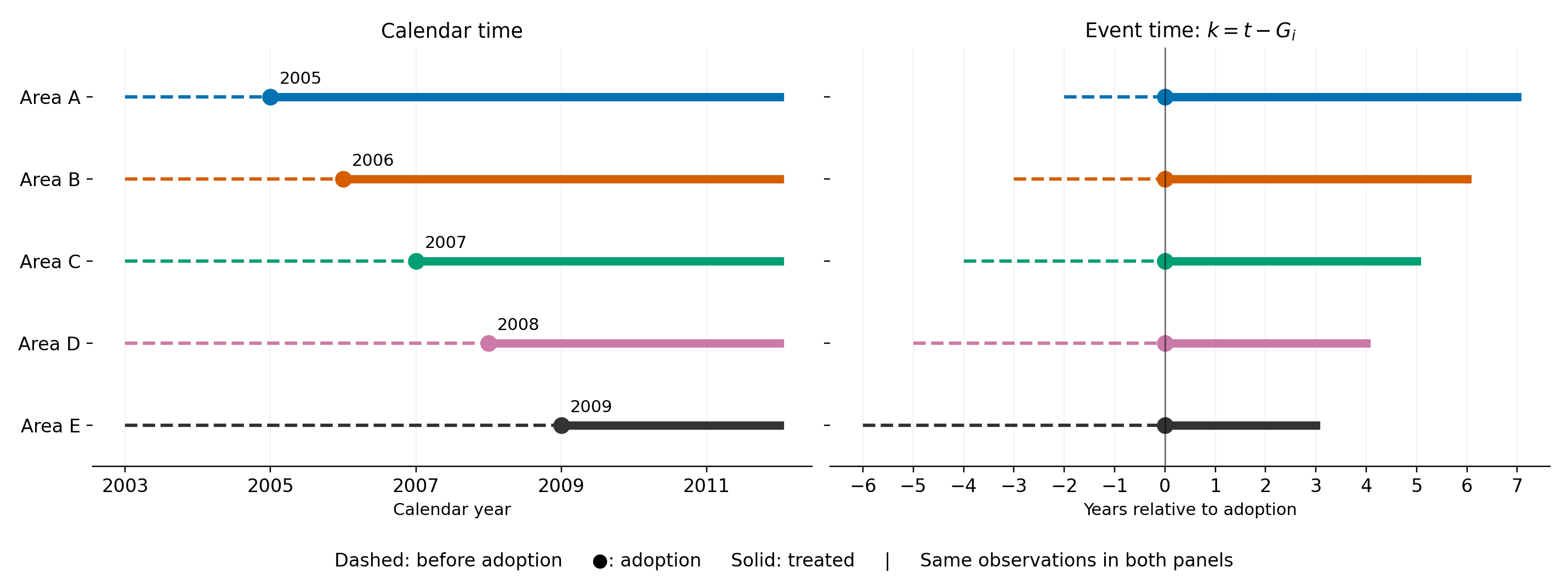
![Five areas observed from 2003 to 2012, adopting between 2005 and 2009. The same rows are shifted so each adoption date is event time zero.]()
In calendar year 2008, Area A is at k=3 and Area E is at k=-1.
From One Post Indicator to Period Indicators
For this introduction, the treated group adopts in the same year G.
Replace the single interaction T_i\cdot Post_t with a separate interaction for each period:
T_i\cdot\mathbf{1}\left(t-G=k\right).
- T_i=1 identifies membership in the treatment group.
- \mathbf{1}\left(t-G=k\right)=1 in the particular period k relative to adoption.
- Their product equals one for a treated-group observation in that period.
What the Dummy Variables Look Like
One treated unit, adopting in G=2007 (T_i=1 throughout):
| 2006 |
-1 |
0 |
0 |
0 |
0 |
| 2007 |
0 |
1 |
1 |
0 |
0 |
| 2008 |
1 |
1 |
0 |
1 |
0 |
| 2009 |
2 |
1 |
0 |
0 |
1 |
Treatment stays on. Each period indicator selects one particular year.
The Event-Study Regression
Y_{it}=\alpha_i+\lambda_t+
\sum_{\substack{k=-K\\k\ne-1}}^{L}\beta_k\left(T_i\cdot\mathbf{1}\left(t-G=k\right)\right)+u_{it}.
- \alpha_i: unit fixed effects.
- \lambda_t: calendar-period fixed effects.
- k=-1: the omitted reference period.
- \beta_k: the treatment–control gap in period k, relative to that gap at k=-1.
Why Omit a Period?
Across the full observation window,
\sum_{k=-K}^{L}T_i\cdot\mathbf{1}\left(t-G=k\right)=T_i.
T_i is already explained by the unit fixed effects. Including every event-time indicator creates perfect multicollinearity.
Set \beta_{-1}=0 by omitting that indicator.
The reference point is zero by construction. It has no estimated confidence interval.
A Coefficient Is a Difference-in-Differences
Write \bar Y_{1,k} and \bar Y_{0,k} for the treated and control means at event time k.
\widehat\beta_k=
\left(\bar Y_{1,k}-\bar Y_{0,k}\right)
-\left(\bar Y_{1,-1}-\bar Y_{0,-1}\right).
Under parallel trends and no anticipation, post-treatment coefficients estimate effects on the treated at each horizon.
Pre-treatment coefficients describe changes in the group gap before treatment.
Reading an Event-Study Graph
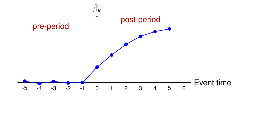
![Original lecture illustration: near-zero pre-treatment coefficients and rising post-treatment coefficients.]()
This schematic illustrates the coefficient pattern. Empirical graphs also need uncertainty intervals.
Leads and Lags
Leads: coefficients for pre-treatment event times, excluding the reference period.
Lags: coefficients for post-treatment periods, with k=0 marking treatment onset.
When reading an empirical graph, identify:
- The outcome and its units.
- The omitted period and treatment date.
- The estimates and confidence intervals.
- The periods and units contributing to each point.
What Do Pre-Treatment Coefficients Test?
A changing pre-treatment gap can reflect:
- Different underlying trends.
- Anticipation of treatment.
- Changes in sample composition.
- An inappropriate regression specification.
Sampling variation also matters. Examine both the pattern and its uncertainty.
Joint Tests of Pre-Trends
A common null hypothesis is
H_0:\beta_{-K}=\cdots=\beta_{-2}=0.
- A joint test assesses the pre-treatment coefficients together.
- Rejection challenges the proposed comparison or treatment timing.
- Failure to reject can reflect low statistical power.
Combine the test with the graph and knowledge of the setting.
Choosing the Time Window
A longer pre-period gives more evidence about the comparison.
A shorter window may describe more comparable circumstances.
Explain the choice using the setting, then investigate how the conclusion changes under plausible alternatives.
Selecting a window because its pre-trend test passes can distort subsequent inference.
Anticipation and Treatment Dynamics
Treatment may affect behaviour before its official implementation date.
- Announcement may induce early responses.
- Implementation may be gradual.
- Outcomes may respond with a delay.
For fertility, conception and birth occur at different dates. Match the event clock to the mechanism.
Binning Distant Periods
Researchers sometimes combine endpoint periods, for example
T_i\cdot\mathbf{1}\left(t-G\leq-5\right),\qquad
T_i\cdot\mathbf{1}\left(t-G\geq5\right).
The final point then represents several periods.
Check what each point contains. With staggered adoption, distant horizons may also contain fewer cohorts.
Healthcare and Fertility: The Policy
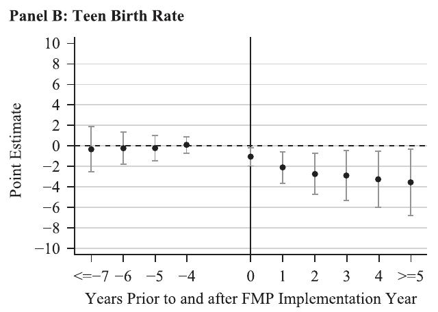
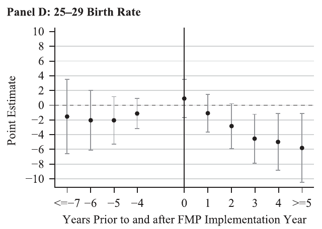
Cesur, Güneş, Tekin and Ulker (2023) study Turkey’s Family Medicine Program.
- Each citizen was assigned a family physician providing free primary care at neighbourhood clinics.
- Services included reproductive health and family planning.
- Adoption spread across provinces from 2005 to 2010.
For discussion: Why might this policy change fertility? Would you expect the response to be immediate or gradual?
Healthcare and Fertility: Data and Identification
- Province-year data, 2001–2018, covering all 81 provinces.
- Outcomes: births per 1,000 women, separately by age group.
- Treatment: introduction of the Family Medicine Program.
- Compare changes across provinces adopting at different dates.
For discussion: What must be true of the timing of adoption for these comparisons to identify a causal effect? Which differences can province fixed effects absorb?
16 and Pregnant: The Question
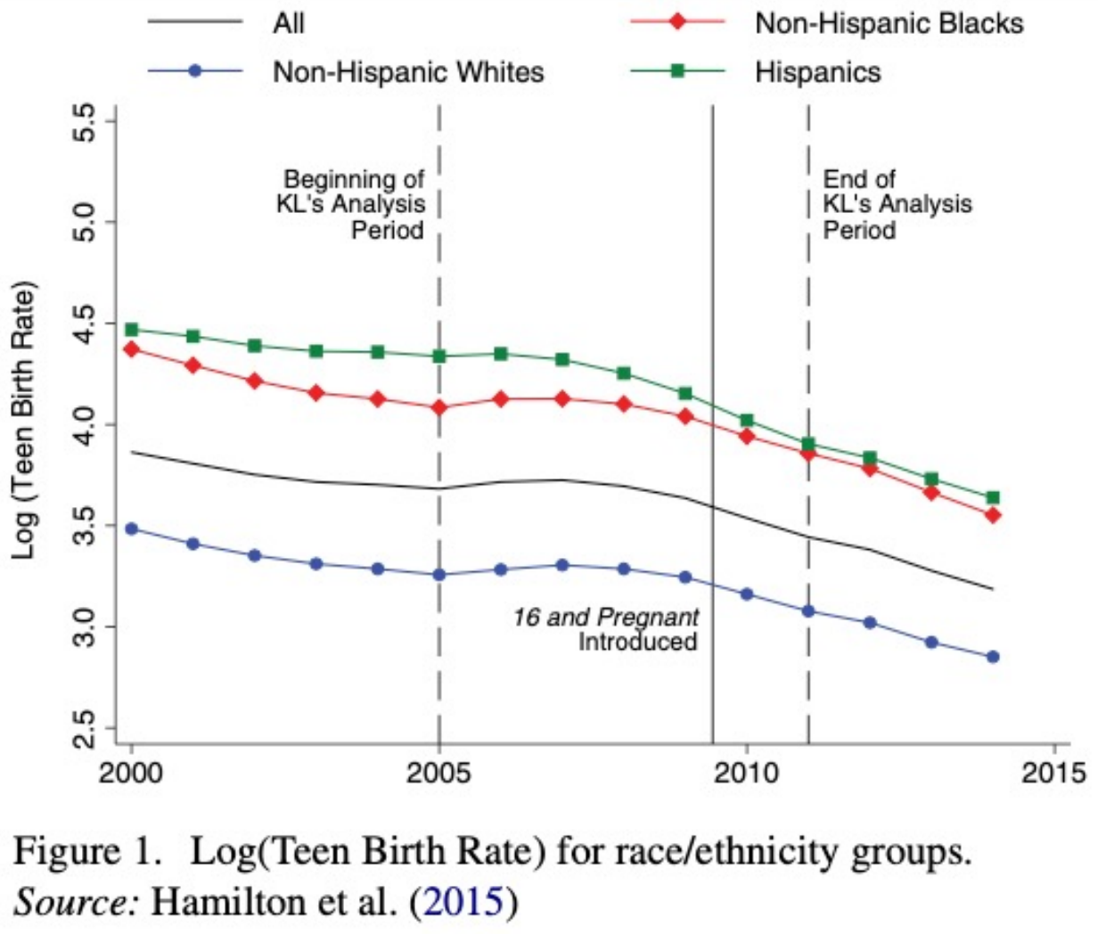
Kearney and Levine (2015) examine whether exposure to MTV’s 16 and Pregnant reduced teenage childbearing.
The programme began broadcasting nationally in 2009, while exposure differed across media markets.
For discussion: Explain the proposed mechanism. What comparison might distinguish the effect of the programme from the existing decline in teenage births?
Data and Identification
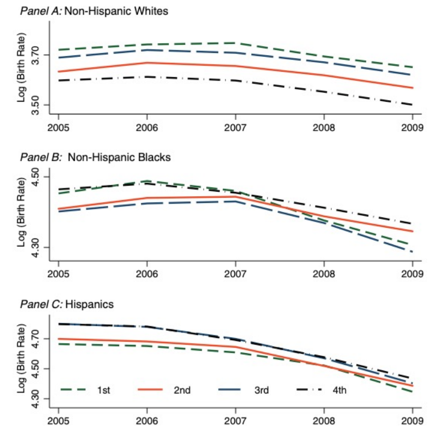
For discussion: Identify the outcome, geographic unit, time period and measure of exposure. Explain how earlier MTV ratings are used as an instrument. What assumptions are required for differences in ratings to identify the programme’s effect?
Exposure and the Post Indicator
Let R_i measure programme exposure and Z_i measure earlier MTV ratings. A simplified representation is
Y_{it}=\alpha_i+\lambda_t+\delta\left(R_i\cdot Post_t\right)
+\sum_j\theta_jX_{jit}+u_{it}.
The instrument for R_i\cdot Post_t is Z_i\cdot Post_t.
The comparison uses differences in exposure across markets, with a common broadcast date.
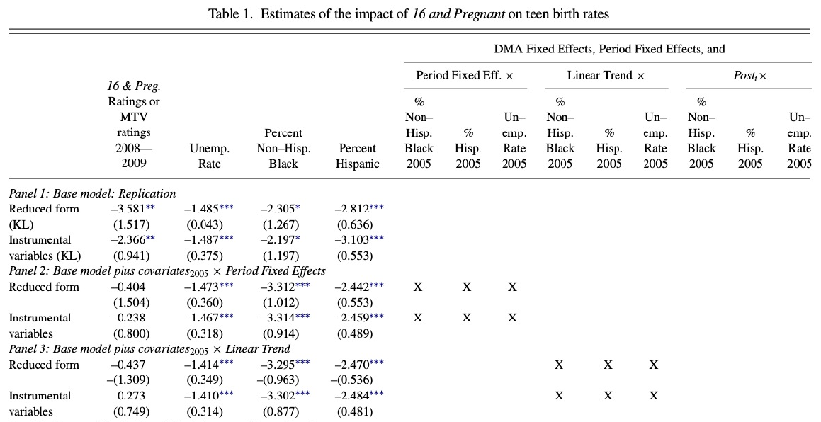
Jaeger, Joyce and Kaestner: Table 1
![JJK Table 1, column headings and Panels 1–3: replication and adjustment for baseline covariates interacted with time.]()
Table 1, Panels 1–3. Source: Jaeger, Joyce and Kaestner (2020). Outcome: 100 × log teen birth rate. Standard errors clustered by DMA. Population-weighted regressions.
For discussion: Compare Panels 1–3. What changes in the specification? Explain the magnitude and uncertainty of the reduced-form and IV estimates.
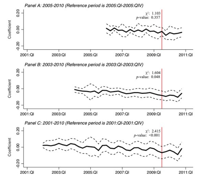
Jaeger, Joyce and Kaestner: Table 5
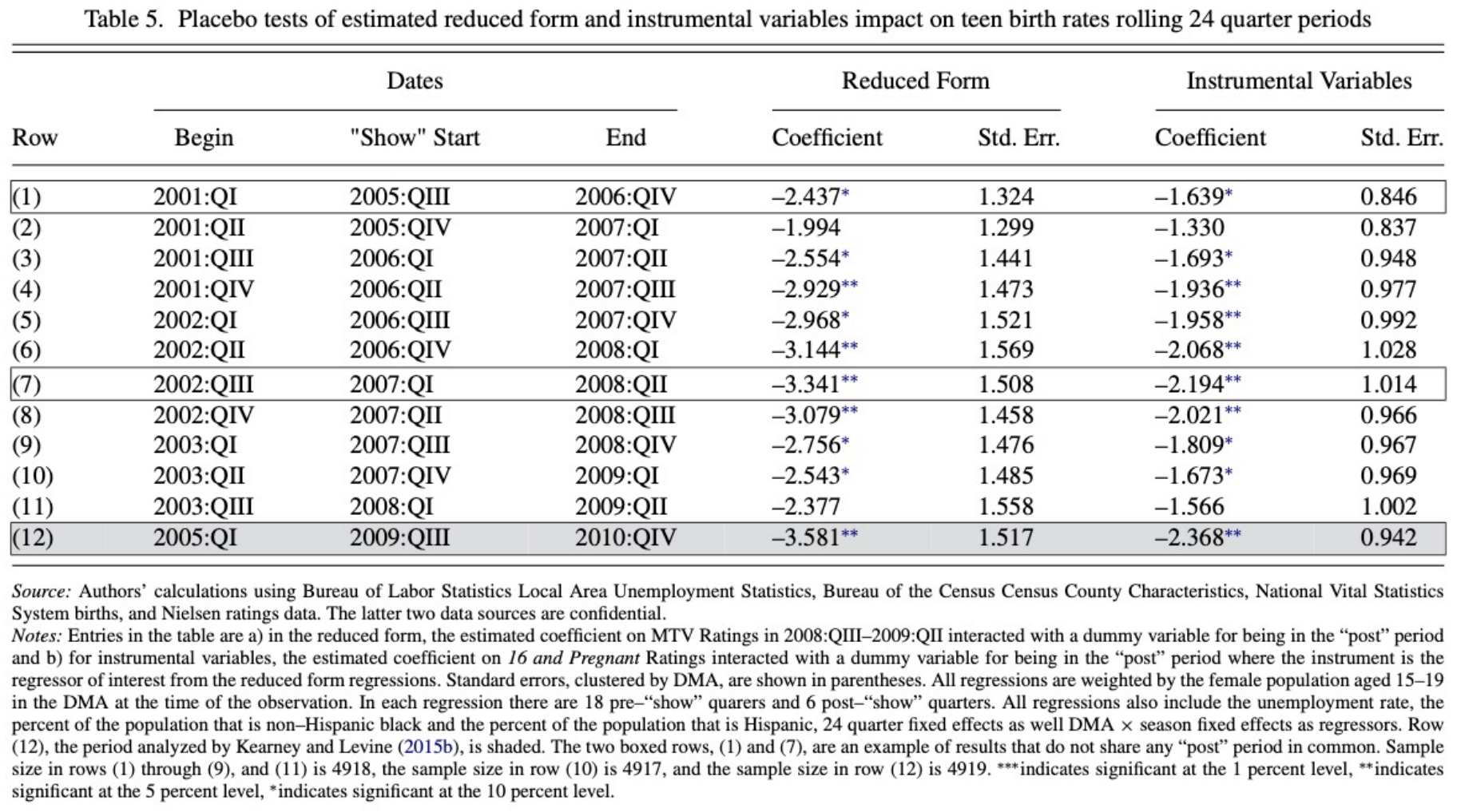
![JJK Table 5: placebo estimates using rolling 24-quarter periods before the actual programme.]()
For discussion: Explain the placebo dates and samples. What would an apparent effect before the programme tell us about the identifying assumptions?
Assessing the Evidence
For discussion: Which evidence most affects your judgement? What would you tell a policymaker considering a media campaign to reduce teenage childbearing?
Distinguish the empirical finding, its identifying assumptions and the policy recommendation.
Different Treatment Dates
For staggered adoption, first-treatment dates differ:
k=t-G_i.
A province three years after adoption may be compared with a province that has already been treated for five years.
If effects change with exposure duration, that comparison needs particular care.
Next week: identify the comparisons conventional TWFE makes, and how modern DiD methods change them.
Reading an Event Study: Checklist
- What is the treatment, comparison and treatment date?
- What is the outcome, in what units?
- Which period is omitted?
- Are pre-treatment estimates informative in both magnitude and precision?
- Is anticipation or a delayed response plausible?
- Are endpoints binned or samples changing across horizons?
- What uncertainty does the design allow us to quantify?
References
Kearney, M. S., and P. B. Levine (2015). Media Influences on Social Outcomes: The Impact of MTV’s 16 and Pregnant on Teen Childbearing. AER 105(12): 3597–3632.
Jaeger, D. A., T. J. Joyce, and R. Kaestner (2020). A Cautionary Tale of Evaluating Identifying Assumptions: Did Reality TV Really Cause a Decline in Teenage Childbearing?. JBES 38(2): 317–326.
Cesur, R., P. M. Güneş, E. Tekin, and A. Ulker (2023). Socialized Healthcare and Women’s Fertility Decisions. JHR 58(3): 1028–1055.
Miller, D. L. (2023). An Introductory Guide to Event Study Models. JEP 37(2): 203–230.