Week 4: IV in Practice — Judges and Examiners
Pre-trial detention and disability insurance
Class slides · Download slides as PDF · Download notes as PDF · Download Quarto source · After-class exercise
Learning Objectives
By the end of this topic, you should be able to:
- Explain how the assignment of cases to judges or examiners can generate quasi-random variation in treatment.
- Construct a leave-one-out leniency instrument and explain why the assignment process determines which comparisons are credible.
- Assess relevance, independence, exclusion, and monotonicity using the institutional details and empirical evidence in the papers.
- Interpret the estimated effects for marginal defendants or applicants and assess what they imply for changes in policy.
Before class
Read these notes and both empirical papers below in full. Both papers are available on Moodle. Our discussion will focus on how the institutions generate an instrument, the evidence supporting its assumptions, and the policy interpretation of the estimates. The “Your turn” boxes below contain the discussion questions. Prepare your assigned items individually, using the discussant list on Moodle.
- Dobbie, Goldin, and Yang (2018), “The Effects of Pretrial Detention on Conviction, Future Crime, and Employment: Evidence from Randomly Assigned Judges.” Our class discussion will draw particularly on Figure 1 and Tables 2–5. Published paper.
- Maestas, Mullen, and Strand (2013), “Does Disability Insurance Receipt Discourage Work? Using Examiner Assignment to Estimate Causal Effects of SSDI Receipt.” Our class discussion will draw particularly on the assignment of examiners, Figure 4, Table 2, Tables 4–5, and Figure 6. Published paper.
Textbook references
Revisit the IV assumptions and LATE from Week 3:
- The Effect: Chapter 19, Instrumental Variables.
- Causal Inference: The Remix: Chapter 7, Instrumental Variables.
- Mastering ’Metrics: Chapter 3, Instrumental Variables. Companion resources · Mastering Econometrics videos at Marginal Revolution University.
- Mostly Harmless Econometrics — advanced reading: Chapter 4, particularly the discussion of heterogeneous effects and LATE.
Additional reading: Goldsmith-Pinkham, Hull, and Kolesár (2026), “Leniency Designs: An Operator’s Manual”.
1. How leniency designs generate a comparison
Decisions made by different officials
Many policies give an official discretion over whether someone receives a treatment. The official reviews a case and decides whether to approve an application, grant access to a service, or impose a restriction. Even when officials apply the same formal rules, they can differ in how they assess evidence or interpret a borderline case. An official who grants the treatment more readily is described as more lenient. Here leniency refers to the tendency to grant the particular treatment being studied.
There are therefore two reasons why treatment decisions can differ across people: their cases differ, and the officials deciding their cases differ. The first source raises the selection problem we have discussed throughout the module. Characteristics that influence approval can also influence the outcome. The second source can supply an instrument when the assignment process gives otherwise comparable people different chances of encountering a lenient official.
Where does the quasi-random variation come from?
Imagine an office with two officials who receive applications from the same queue. A central allocation system sends each new application to one of them. Suppose this allocation is unrelated to the applicant’s characteristics or potential outcomes. One official approves 40% of the office’s applicants, while the other approves 60%. These are hypothetical population rates, illustrating a persistent difference in their decisions.
An applicant’s chance of approval then depends partly on which official happens to receive the file. Across many assignments, the two officials receive comparable applicants, including comparable distributions of characteristics the researcher cannot observe. Assignment to the more lenient official raises the probability of treatment by 20 percentage points.
The assignment process supplies the quasi-random comparison. Differences in leniency make that comparison predict treatment. Together they provide the independence and relevance arguments familiar from IV.
An institution might allocate cases by an explicit lottery. In other settings, a rotation, a queue, or the official available when a case arrives may produce an assignment that is plausibly as good as random within a suitable group of cases. The researcher establishes why the actual procedure has this property. For example, a rotation is persuasive if applicants cannot time their arrival to obtain a particular official and case characteristics do not systematically change with the rotation. Preferential allocation of difficult cases to experienced officials would require a different argument and an appropriate comparison group.
The term quasi-random captures this institutional claim: within the comparison being used, who receives the more lenient official is effectively a matter of chance with respect to the determinants of the outcome.
Assignment and treatment selection
For the two-official example, let \(Z_i=1\) mean assignment to the more lenient official and \(Z_i=0\) assignment to the stricter official. Let \(D_i=1\) mean that the applicant receives treatment.
The official still assesses the case. Applicants with stronger claims may be approved by either official, while those with weaker claims may be rejected by either. Thus the treated and untreated groups can differ systematically even when the assigned-official groups are comparable. This is the same distinction we made in Oregon between lottery assignment and obtaining insurance.
We can first compare outcomes by assigned official. With quasi-random assignment, this comparison identifies the effect of assignment. To interpret the difference as operating through treatment, we need the exclusion restriction: the official affects the outcome through the treatment decision. The Wald estimator then scales the outcome difference by the treatment-probability difference. Monotonicity supplies the local treatment-effect interpretation when effects differ across individuals.
Which applicants are comparable?
An office may allocate different categories of cases to different teams. Officials may also serve different locations or shifts. Suppose applicants with more serious conditions go to a specialist team whose members approve applications more often. Comparing that team’s applicants with the rest of the office would combine differences in official leniency with differences in the applicants’ conditions.
The useful comparison would instead be within the teams and periods in which applicants could have been assigned to the same officials. Controls for those assignment groups preserve that comparison in the regression. Their choice follows from how the institution allocates cases.
To assess the argument, establish who can be assigned to whom, whether applicants or staff can influence the assignment, and whether particular officials receive systematically different cases. Balance checks on characteristics measured before assignment provide empirical evidence alongside that institutional description. The argument about unobserved characteristics rests on understanding the assignment process.
This week’s applications
The papers below use these ideas in two settings. As you read, identify the assignment process first, then consider how differences in officials’ decisions change treatment probabilities.
| Pre-trial release | Disability insurance | |
|---|---|---|
| Individual | Defendant | Applicant |
| Treatment, \(D_i=1\) | Released within three days of the bail hearing | Receives SSDI benefits |
| Instrument, \(Z_i\) | Assigned bail judge’s release tendency, estimated using other defendants | Assigned examiner’s initial allowance rate, estimated using other applicants |
| Examples of \(Y_i\) | Conviction, guilty plea, employment | Employment, earnings |
Treatment coding matters: the detention paper’s principal regressions estimate the effect of release. A negative coefficient on release corresponds to a positive effect of detention for the same comparison.
The assumptions in this setting
- Relevance: assignment to a more lenient official changes the probability of treatment.
- Independence, conditional on assignment controls: within the relevant assignment groups, the official assigned is unrelated to potential outcomes and potential treatment decisions.
- Exclusion: changing the assigned official affects the outcome through treatment.
- Monotonicity: moving from a stricter to a more lenient official moves treatment decisions in a common direction for individuals.
We also retain the treatment definitions and no-interference conditions discussed under SUTVA. For example, if one official’s decisions change the resources available for other cases, we should consider whether those spillovers matter for the comparison.
In the linear model, the assignment and exclusion arguments support the orthogonality condition for IV. With heterogeneous effects, the additional monotonicity argument gives the estimates a local treatment-effect interpretation.
2. Measuring leniency
Suppose official \(j\) handles \(n_j\) cases. Write \(R_i=1\) when the official makes a favourable initial decision for person \(i\). The official’s average decision rate includes \(R_i\) itself. Thus a person’s own circumstances help determine both their decision and this average.
We instead calculate the official’s favourable-decision rate among other cases:
\[Z_i=\frac{\sum_{k:j(k)=j(i),\ k\ne i}R_k}{n_{j(i)}-1}.\]
Here \(j(i)\) denotes the official assigned to person \(i\). This is a leave-one-out measure: we exclude person \(i\) when measuring the leniency of their assigned official.
For example, an official approves three of five cases. For an approved applicant, the leave-one-out rate is \(2/4=0.50\). For a rejected applicant, it is \(3/4=0.75\). Each applicant’s instrument uses the decisions on the other four cases. Within this official’s five cases, approved applicants therefore have a lower leave-one-out value (0.50) than rejected applicants (0.75). This happens because the calculation removes an approval for the former and a rejection for the latter. The useful first-stage variation comes from differences in underlying leniency across officials.
The administrative details determine how this calculation is implemented. Dobbie, Goldin, and Yang first remove court-and-time effects from release decisions, then calculate judge-year averages excluding all cases belonging to the same defendant. Maestas, Mullen, and Strand use other applicants’ initial allowance decisions to instrument eventual benefit receipt, allowing for appeals and subsequent decisions.
Why do we need to leave out individual \(i\) when constructing the instrument for the \(i\)th observation?
Accounting for the assignment process
If different kinds of cases are assigned to different offices, shifts, or specialists, compare cases within the groups for which assignment is plausibly as good as random. The corresponding controls belong in the first stage, reduced form, and outcome equation.
Using our notation, the first stage is
\[D_i=\pi_0+\pi_1 Z_i+\sum_{k=1}^{K}\pi_{k+1}X_{ki}+v_i,\]
and the reduced form is
\[Y_i=\delta_0+\delta_1 Z_i+\sum_{k=1}^{K}\delta_{k+1}X_{ki}+e_i.\]
The \(X_{ki}\) include the assignment controls. With one excluded instrument and one endogenous explanatory variable, the model is exactly identified. Using the same observations and controls in both regressions,
\[\widehat\beta_1^{IV}=\frac{\widehat\delta_1}{\widehat\pi_1}.\]
The first stage regresses the endogenous explanatory variable on all the exogenous variables. The reduced form regresses the outcome on all the exogenous variables.
3. Pre-trial detention
Policy question and data
Dobbie, Goldin, and Yang study bail hearings in Philadelphia and Miami-Dade, linking court records to administrative tax records. Detention can affect several policy outcomes at once: appearance in court, subsequent arrests, the resolution of the current case, and employment.
What decision is being evaluated? Explain the treatment and outcome variables. Why might defendants released before trial have different outcomes from detained defendants even if release had no causal effect? Which outcomes would you want a policy evaluation to consider?
Assignment and balance
Bail judges work rotating schedules. The comparison accounts for court and time of the hearing. Philadelphia’s shift system requires additional attention to time of day. The paper explains why defendants generally have limited ability to choose their bail judge, while also discussing possible selection in who reaches a hearing.
The balance exercise compares two relationships: the association of observed characteristics with actual release, and their association with the assigned judge’s leniency. These answer distinct questions about treatment selection and instrument assignment.
Use the institutional description and Table 3. How is a judge assigned? Which comparisons require controls for place or time? Explain what the two columns tell us. What concerns would remain even if the observed characteristics were balanced across the instrument?
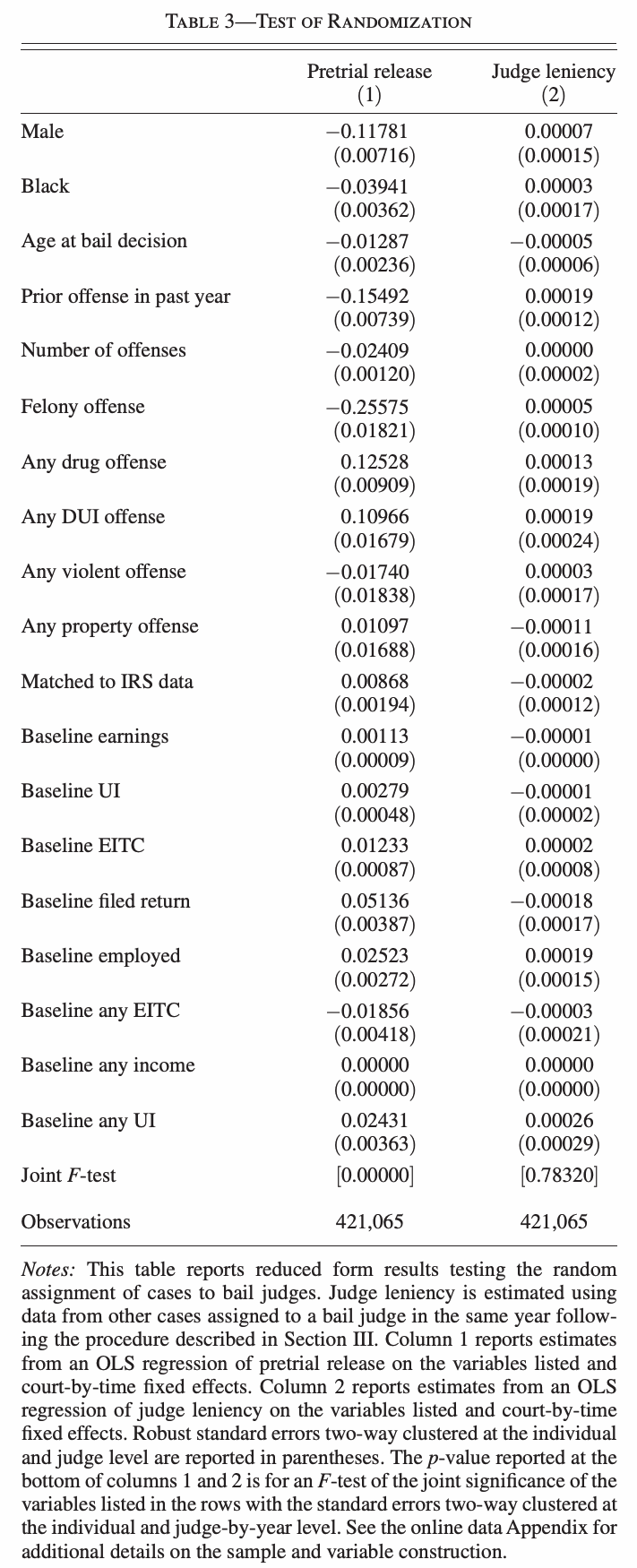
Balance provides evidence about the assignment process. Independence also requires an argument about characteristics we cannot observe. Relate the empirical check to the way cases arrive and judges rotate.
Relevance
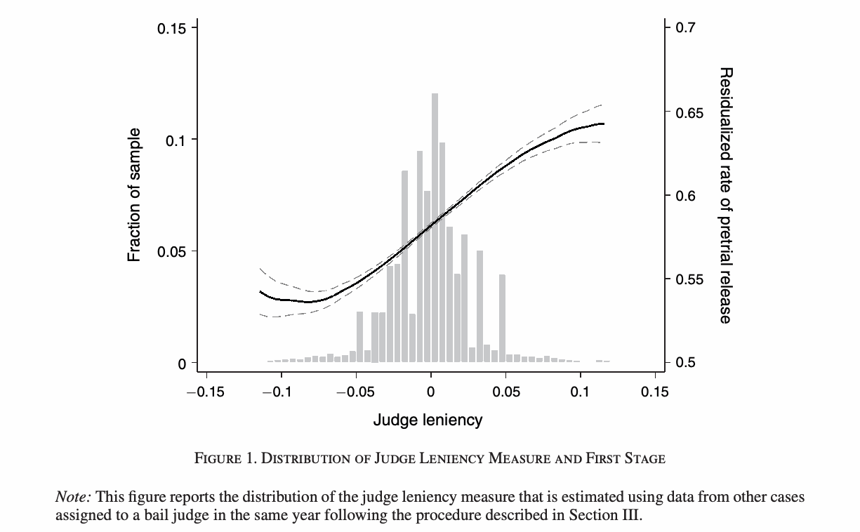
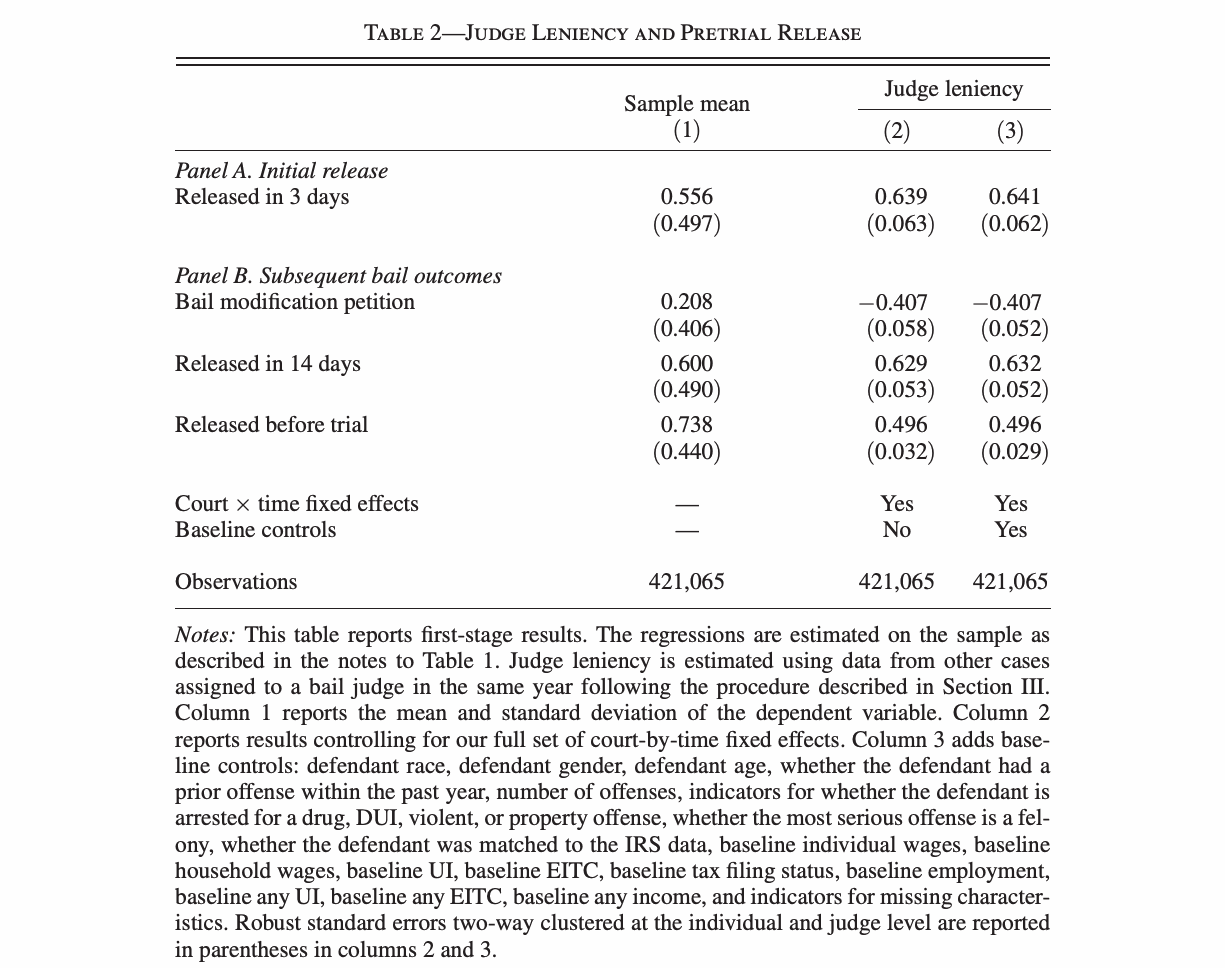
Use Figure 1 and Panel A of Table 2. Identify the axes in the figure and the dependent variable in the table. What does a 0.10 increase in judge leniency predict for the probability of release? Explain why the first-stage coefficient need not equal one.
Exclusion and monotonicity
Why does it matter that bail judges and trial judges are assigned through different processes? Could bail conditions affect later outcomes through a channel besides whether the defendant is released? Describe a pair of defendants for whom judges might reverse their ranking in leniency. Which IV assumption would that challenge?
A useful way to assess exclusion is to list everything the assigned official can change. If a judge changes financial conditions, supervision, or another aspect of the defendant’s experience that independently affects the outcome, a binary release indicator may not capture the full effect of assignment. The separation of bail and trial responsibilities helps address a different concern: the possibility that the instrument also assigns a more lenient decision-maker at conviction or sentencing.
Monotonicity concerns individuals’ potential decisions. A judge with a higher average release rate could still be stricter for a particular type of case. Evidence that first stages are positive across observed groups is useful when assessing this assumption. The underlying requirement concerns how the same defendant would be treated by different judges.
Results and policy interpretation
Use Tables 4 and 5, focusing on the OLS estimate with baseline controls and the corresponding 2SLS estimate (columns 3 and 6). Interpret the effects on guilty pleas, rearrest, and employment. State the units and describe uncertainty. How might release influence a defendant’s willingness to plead guilty? Which policy trade-offs emerge across the outcomes?
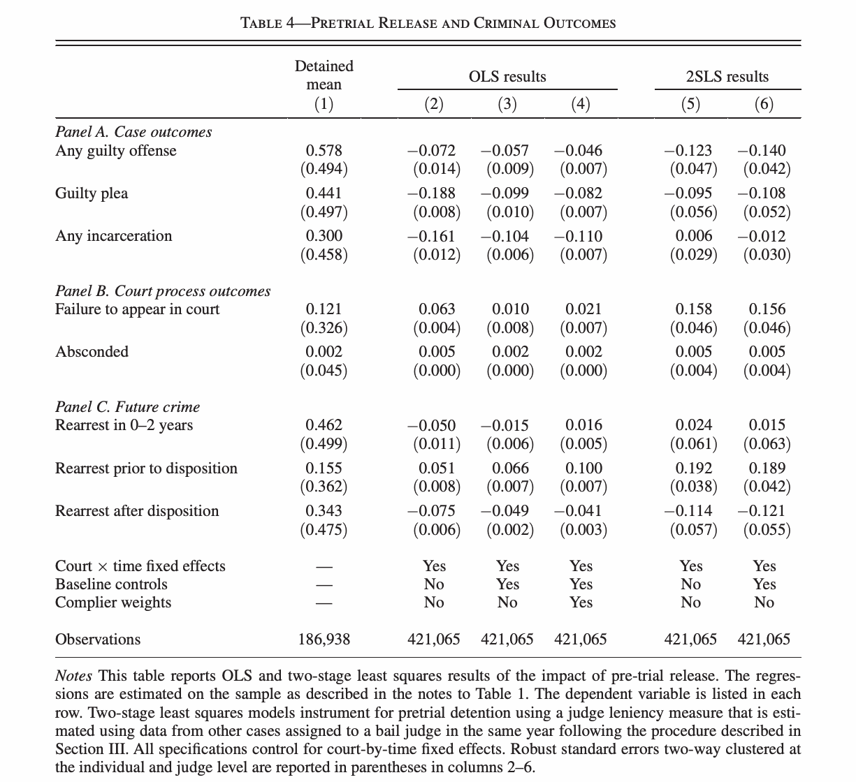
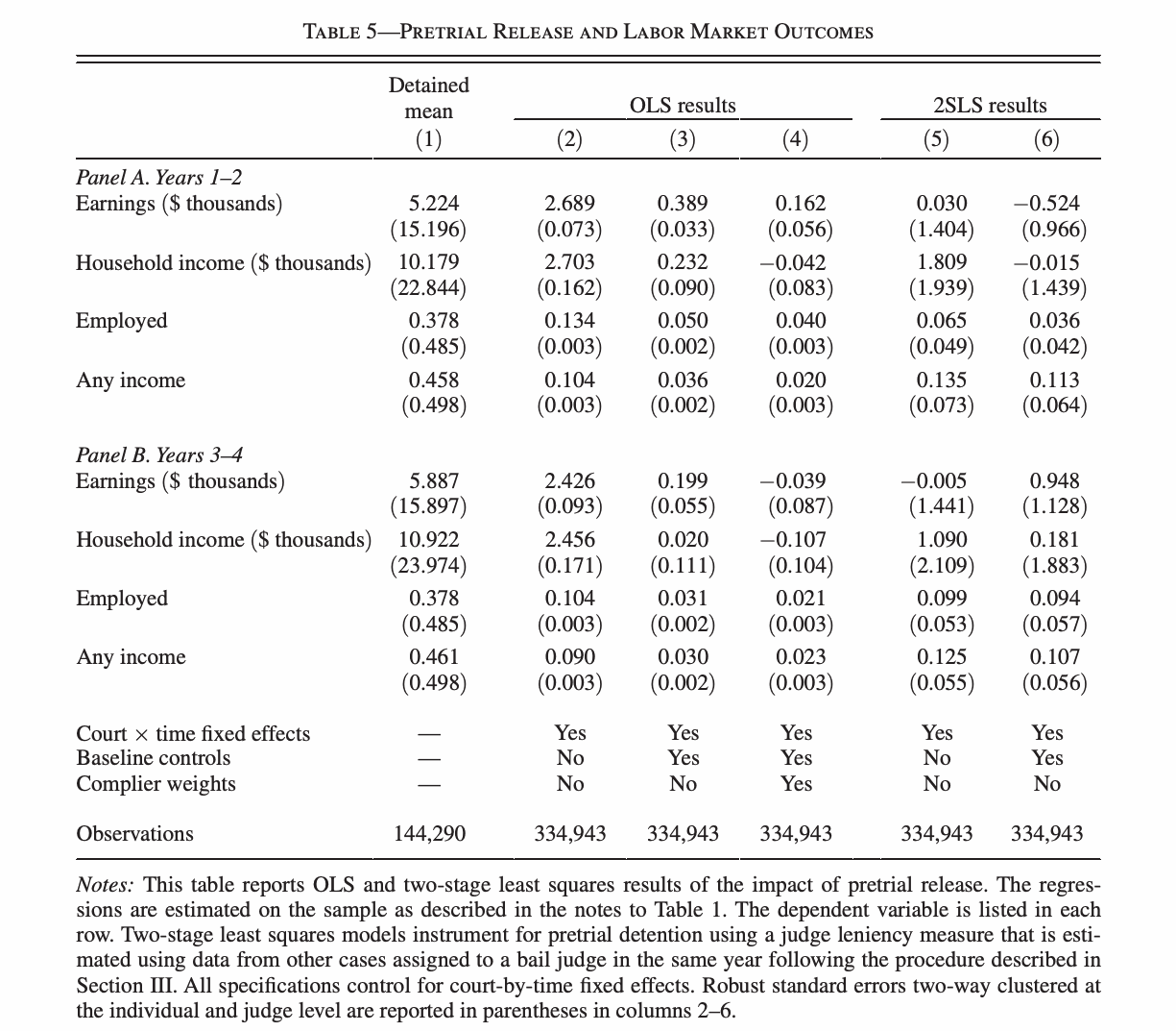
The IV comparison concerns defendants whose release depends on the assigned judge. A proposal to release all defendants would extend beyond that margin. OLS and IV can also differ because the treatment effects vary across defendants and the estimators put weight on different comparisons.
4. Disability insurance
Policy question and assignment
Maestas, Mullen, and Strand study the US Social Security Disability Insurance programme. Benefit receipt can reduce the incentive to work, while applicants’ health limitations affect both their chance of approval and their ability to work. Their administrative data connect applications, assigned examiners, decisions, and subsequent earnings.
Why is employment among rejected applicants informative about the policy question? Why might a comparison of approved and rejected applicants misstate the effect of benefits? Explain the distinction between an initial allowance decision and eventual benefit receipt.
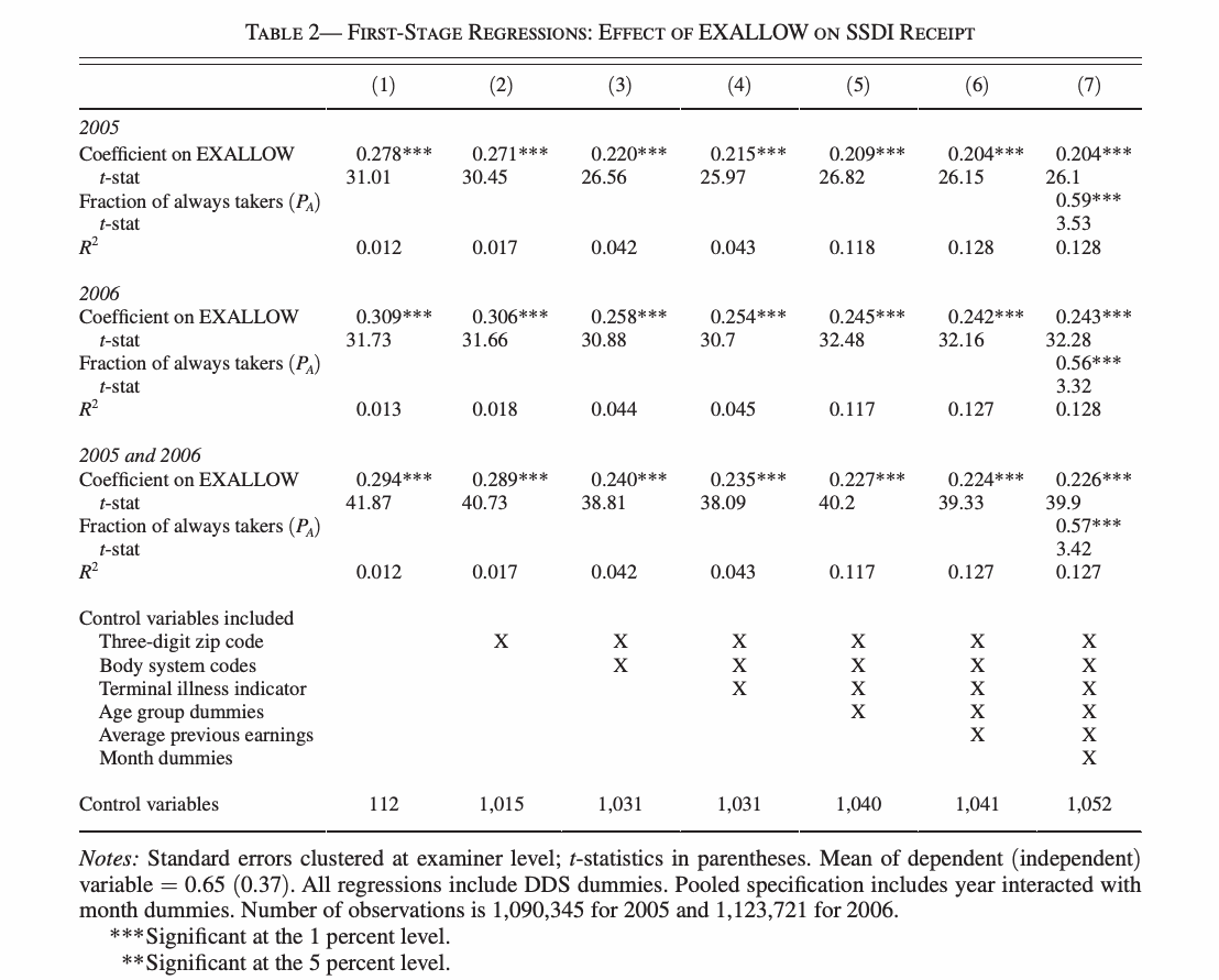
Applicants are assigned within state Disability Determination Services (DDS) offices. Assignment can reflect impairment categories or terminal illness. The authors therefore include office indicators and observed assignment characteristics. Table 2 adds further controls, allowing readers to see how the first stage changes.
Use the institutional description and Table 2. Why are DDS office controls necessary? Which applicant characteristics can affect assignment? What do changes across columns suggest about the relevant comparisons? Explain why unconditional comparisons across all examiners would be problematic.
First stage, reduced form, and IV
Explain both panels of Figure 4. Identify which panel shows the first stage and which shows the reduced form. What sign would you expect for the IV estimate? Use Table 2, column 7, and Table 5 to calculate the estimate for employment two years after a 2005 decision.
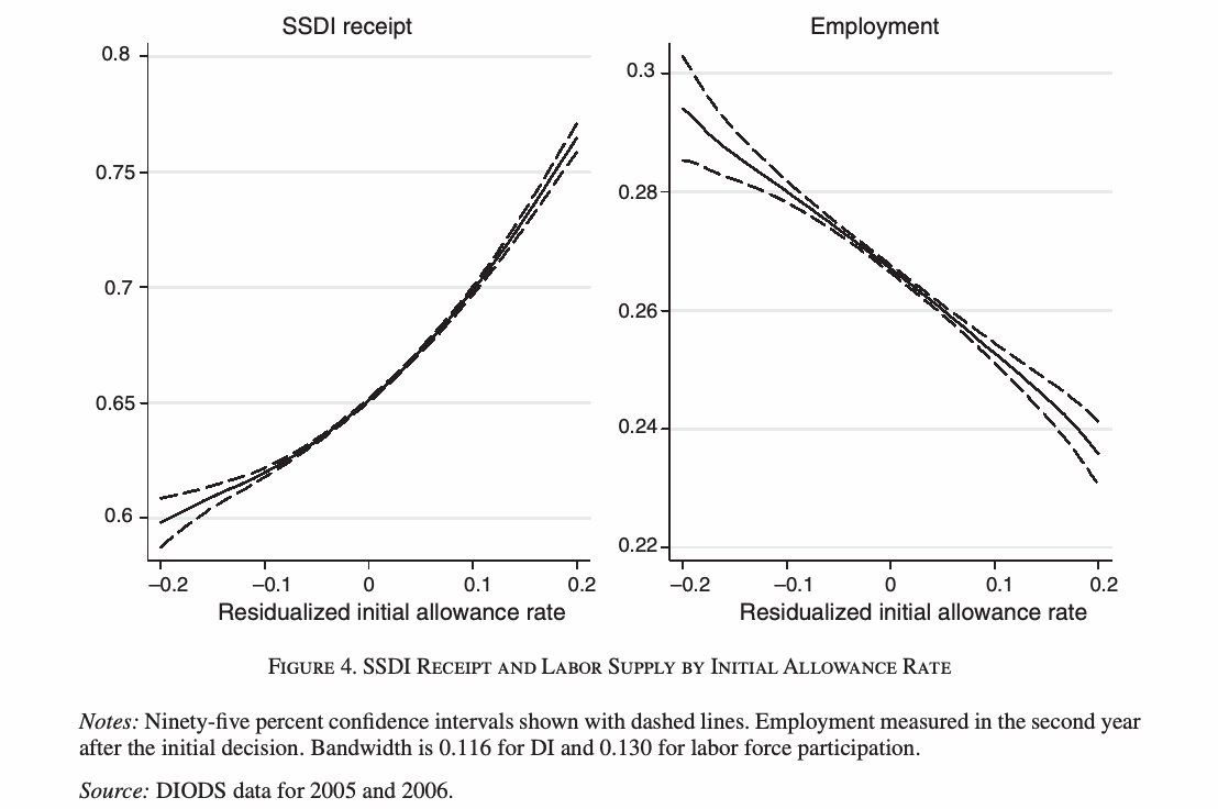
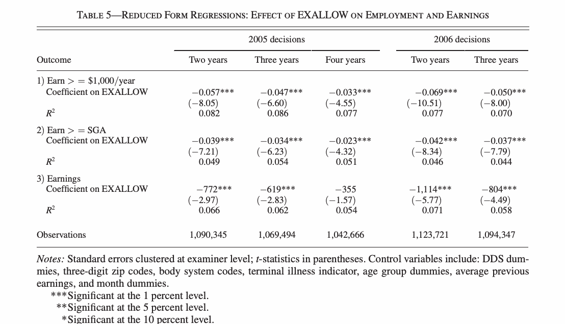
The first-stage coefficient for the 2005 cohort is 0.204, and the reduced-form coefficient for employment two years later is −0.057. Their ratio is approximately −0.279, or a 27.9 percentage-point reduction in employment for the applicants whose benefit receipt is affected by examiner assignment. Small rounding differences arise because the published coefficients are rounded.
Interpreting the effect
For a test of a zero coefficient, \(t=\widehat\beta/\operatorname{SE}\left(\widehat\beta\right)\). Rearranging gives \(\operatorname{SE}\left(\widehat\beta\right)=\left|\widehat\beta\right|/\left|t\right|\). Published rounding makes the recovered standard error approximate.
Focus on Panel A, employment two years after the decision. Compare OLS and IV. Explain the employment definition and the magnitude of the estimated effect. The parentheses contain t-statistics: how would you recover an approximate standard error? Who are the applicants whose treatment status changes with examiner assignment?
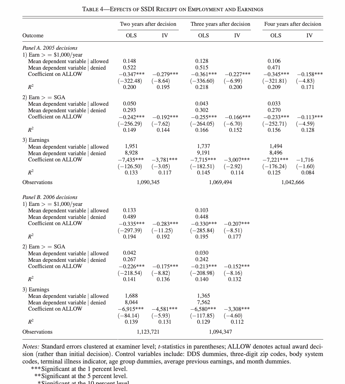
Employment here means annual earnings of at least $1,000. The local effect refers to applicants at the margin of receiving benefits under the observed examiner assignments. A reduction in employment is one consequence to consider alongside the insurance and income protection the programme provides. An overall recommendation also requires evidence about those benefits and the consequences of changing eligibility.
Processing times and exclusion
Use Figure 6. Distinguish initial and final processing times. How might time spent waiting affect later employment? Explain how this bears on interpreting the IV coefficient as the effect of benefit receipt. Read the authors’ discussion of the direction of the resulting bias and their sensitivity calculation.
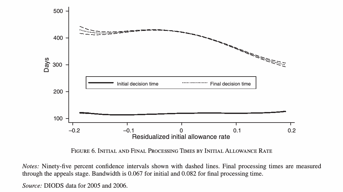
Appeals can lengthen the application process. If assignment affects time out of work as well as benefit receipt, and that waiting time affects subsequent employment, the exclusion argument must address this pathway. The paper discusses it explicitly. Under the proposed mechanism, stricter examiners can lengthen waiting and reduce subsequent employment through skill depreciation. This offsets some of the negative reduced-form effect of greater leniency operating through increased benefit receipt, making the estimated employment reduction from benefits smaller in magnitude than it would otherwise be.
5. Whose effect, and which policy?
To connect this week’s designs to Week 3, temporarily imagine just two officials: a stricter official (\(Z_i=0\)) and a more lenient official (\(Z_i=1\)). A complier receives treatment under the more lenient official but not under the stricter official:
\[D_i^1=1,\qquad D_i^0=0.\]
Under the IV assumptions, the binary-instrument comparison identifies
\[E\left[Y_i^1-Y_i^0\mid D_i^1>D_i^0\right].\]
With many officials and a leniency measure, the estimates combine comparisons across levels of leniency. Under a common monotone ordering, they can be interpreted as weighted averages of effects for individuals whose treatment changes along those margins. The identity of these individuals depends on the officials and assignment process in the study.
A higher average approval rate alone does not establish a common ordering. For example, examiner A could be more willing than examiner B to approve musculoskeletal claims but less willing to approve mental-health claims. This is why the institutional case for monotonicity deserves discussion.
For each paper, give the strongest institutional argument for independence, the most plausible alternative channel threatening exclusion, and a concrete description of the people at the treatment margin. Then propose a policy change to which the estimate is informative. Explain what further evidence would be needed for a broader reform.
A note on standard errors
Individuals assigned to the same official share a source of variation. The papers allow for dependence within relevant groups when calculating uncertainty: Maestas, Mullen, and Strand cluster by examiner. Dobbie, Goldin, and Yang use two-way clustering by defendant and judge. Heteroskedasticity-consistent standard errors address differences in error variances. Clustered standard errors additionally allow errors to be related within the specified groups. We will return to the implications for inference as we use designs with grouped assignment.
6. After-class exercise
Exercise instructions · Download the Quarto notebook
The notebook supplies Python code that generates applicants randomly assigned to caseworkers with different approval thresholds. Each student generates a fresh sample, with no fixed random seed. Construct the leave-one-out instrument, examine the first stage and reduced form, and estimate OLS and IV. Compare your estimates with the known causal effect and explain any differences. This exercise is ungraded.
References
- Dobbie, Will, Jacob Goldin, and Crystal S. Yang. 2018. “The Effects of Pretrial Detention on Conviction, Future Crime, and Employment: Evidence from Randomly Assigned Judges.” American Economic Review 108(2): 201–240.
- Maestas, Nicole, Kathleen J. Mullen, and Alexander Strand. 2013. “Does Disability Insurance Receipt Discourage Work? Using Examiner Assignment to Estimate Causal Effects of SSDI Receipt.” American Economic Review 103(5): 1797–1829.
- Goldsmith-Pinkham, Paul, Peter Hull, and Michal Kolesár. 2026. “Leniency Designs: An Operator’s Manual.” Journal of Economic Perspectives 40(3): 213–240.