Modern Difference-in-Differences
PP5001 · Week 10 · Martinmas 2026
Professor David A. Jaeger
Recall: Two-Way Fixed Effects
Y_{it}=\alpha_i+\lambda_t+\delta D_{it}+u_{it}.
- \alpha_i: time-invariant differences between units.
- \lambda_t: common changes in calendar time.
- D_{it}: whether unit i is treated in period t.
With different adoption dates, which comparisons determine \widehat\delta?
Multiple Treatment Times
Policies often begin in different places at different times:
- Minimum-wage increases.
- Health-insurance expansions.
- School reforms.
- Environmental regulations.
A cohort is a group of units first treated in the same calendar period.
Timing Groups
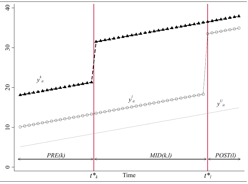
![]()
Timing groups, from the original lecture slides.
For discussion: Identify the early-treated, late-treated and never-treated groups. When can each group supply untreated observations?
Four Comparisons
With early, late and never-treated groups, TWFE combines:
- Early treated versus never treated.
- Late treated versus never treated.
- Early treated versus late treated, before the late group adopts.
- Late treated versus early treated, after the early group has adopted.
In comparison 4, the comparison group’s outcomes already include treatment effects.
The Goodman-Bacon Decomposition
For the basic TWFE regression in a balanced panel,
\widehat\delta^{TWFE}=\sum_j s_j\widehat\delta_j^{2\times2},
\qquad s_j\ge0,\qquad \sum_j s_j=1.
- Each component is a two-group, two-period comparison.
- Timing and treatment variation determine the weights.
- Both not-yet-treated and already-treated groups can serve as controls.
When a Common Effect Is Adequate
Suppose untreated outcomes follow parallel trends and there is no anticipation.
If treatment has the same constant effect for every treated cohort and period, an already-treated group’s treatment effect cancels when its outcome is differenced.
The difficulty arises when that effect changes over the comparison period.
An Illustration
Suppose every group’s untreated outcome would remain at 10.
| Early treated |
10 |
12 |
16 |
| Late treated |
10 |
10 |
12 |
| Never treated |
10 |
10 |
10 |
Early adopters have an effect of 2 initially and 6 later. Late adopters have an effect of 2 when they adopt.
The Same Illustration Graphically
![]()
For discussion: From period 1 to period 2, whose observed outcome changes most? What would happen if we used that group as the control for late adopters?
Using an Untreated Comparison
From period 0 to period 1:
\widehat\delta_{Early,Late}=(12-10)-(10-10)=2.
From period 1 to period 2, using never-treated units:
\widehat\delta_{Late,Never}=(12-10)-(10-10)=2.
Each calculation recovers the newly treated group’s effect.
Using an Already-Treated Comparison
Compare late with early adopters from period 1 to period 2:
\widehat\delta_{Late,Early}=(12-10)-(16-12)=-2.
The late group’s treatment effect is +2, but this comparison subtracts the +4 change in the early group’s treatment effect.
For discussion: Why does a negative comparison arise even though every treatment effect is positive?
What Is Being Subtracted?
Under parallel trends in untreated outcomes,
DiD_{Late,Early}
=\text{late group's new effect}
-\text{change in early group's effect}.
Growing effects in the early cohort reduce this component of TWFE.
Weights on Treatment Effects
The weights on the component 2\times2 comparisons are positive.
But an already-treated comparison subtracts changes in treatment effects. When TWFE is expressed in terms of underlying cohort-period effects, some of those effects can receive negative weight.
A TWFE coefficient can consequently lie outside the range of the underlying treatment effects.
Event-Study Coefficients
In a conventional TWFE event study with staggered adoption:
- Units at different event times are observed in the same calendar period.
- Treatment effects can differ across cohorts and exposure lengths.
- An estimated lead or lag can combine effects from other event times.
Even an apparent pre-treatment coefficient can reflect post-treatment effects elsewhere.
Make the Comparisons Explicit
The approach we will use has three steps:
- Define an untreated comparison group.
- Estimate effects separately for each adoption cohort and calendar period.
- Average those effects to answer a stated policy question.
Callaway and Sant’Anna (2021) organise their method around these steps.
A Group-Time Treatment Effect
Let G_i=g mean that unit i first receives treatment in period g.
ATT(g,t)=E\left[Y_{it}^{g}-Y_{it}^{\infty}\mid G_i=g\right],\qquad t\ge g.
- Y_{it}^{g}: outcome at t if treatment first begins at g.
- Y_{it}^{\infty}: outcome at t if the unit remains untreated.
- ATT(g,t): effect at t for the cohort first treated at g.
Reading the Two Dates
ATT(2004,2006)
means the effect in calendar year 2006, for units first treated in 2004.
Their event time is
k=t-g=2006-2004=2.
For discussion: Which effect would describe the 2006 cohort in its first treatment year? Which would describe that same cohort one year later?
Identify the Counterfactual
Use g-1, the last pre-treatment period, as the baseline.
With never-treated units as controls, assume
E\left[Y_{it}^{\infty}-Y_{i,g-1}^{\infty}\mid G_i=g\right]
=E\left[Y_{it}^{\infty}-Y_{i,g-1}^{\infty}\mid G_i=\infty\right].
Also assume no anticipation at the baseline.
Back to a Two-by-Two Difference
Under those assumptions,
\begin{aligned}
ATT(g,t)={}&E\left[Y_{it}-Y_{i,g-1}\mid G_i=g\right]\\
&-E\left[Y_{it}-Y_{i,g-1}\mid G_i=\infty\right].
\end{aligned}
The sample estimator replaces each expectation with its corresponding sample mean.
We already know how to calculate this comparison.
Choosing the Comparison Group
Never treated: remain untreated throughout the observation period.
Not yet treated: remain untreated through the outcome period t.
For the latter, use units with G_i>t, including never-treated units where available, and maintain the corresponding parallel-trends and no-anticipation assumptions.
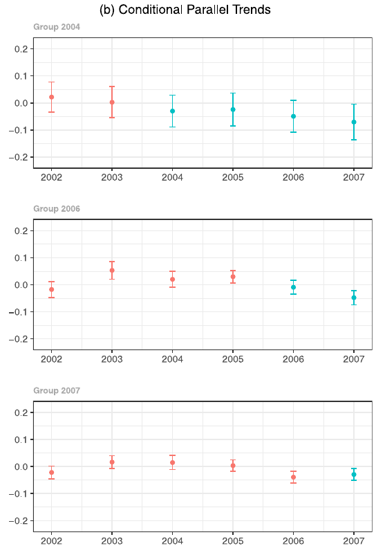
Conditional Parallel Trends
Sometimes parallel trends is plausible only among units with similar baseline characteristics X_i.
Estimate comparisons conditional on those characteristics, then average over the treated cohort’s characteristics.
Overlap is needed: the comparison group must contain suitable counterparts for the treated cohort.
Which Average Do We Want?
Once we have ATT(g,t), we can average:
- Within cohorts: how did each adoption cohort fare?
- Within calendar years: what was the effect among treated units in a particular year?
- At a common event time: how does the effect evolve with exposure?
These averages can differ because they combine different effects with different weights.
An Event-Time Average
At event time k\ge0, combine available cohorts at t=g+k:
\theta_k=\sum_{g\in\mathcal G_k}w_{g,k}\,ATT(g,g+k),
\qquad w_{g,k}\ge0,\qquad \sum_{g\in\mathcal G_k}w_{g,k}=1.
\mathcal G_k contains cohorts observed at event time k with a valid comparison group. Cohort-size weights give larger cohorts more influence.
Changing Cohort Composition
Suppose data end in 2007.
An event-time graph can change because effects evolve and because the contributing cohorts change.
A balanced-cohort graph keeps the same cohorts at every displayed exposure length.
Minimum Wages Revisited
Callaway and Sant’Anna study county-level teenage employment during 2001–2007.
- The federal minimum wage stays at $5.15 over the study window.
- Treated states raise their minimum wage above that level.
- Cohorts are defined by the first increase.
- The main comparison group is counties in states that remain at the federal minimum.
For discussion: Explain the policy, data and source of identifying variation. What differs from Card and Krueger’s comparison?
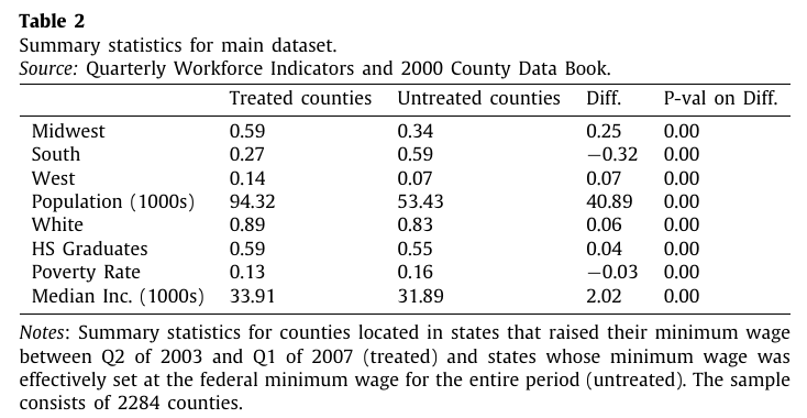
Table 2: The Comparison Groups
![]()
Callaway and Sant’Anna (2021), Table 2, p. 217.
For discussion: Describe the differences between treated and untreated counties. What do these differences imply for the parallel-trends argument and the choice of controls?
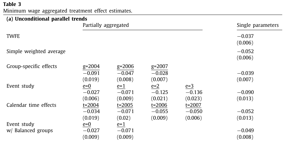
Table 3(a): Different Averages
Callaway and Sant’Anna (2021), Table 3(a), p. 219.
For discussion: Focus on TWFE and the group-specific effects. Compare the TWFE estimate with the overall group-specific effect in the rightmost column. How similar are they?
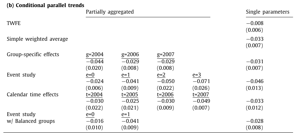
Table 3(b): With Covariate Adjustment
Callaway and Sant’Anna (2021), Table 3(b), p. 219.
For discussion: Compare TWFE with the overall group-specific effect in the rightmost column. What changes relative to panel (a) after covariate adjustment? Would your policy conclusion depend on the estimator?
Assessing the Policy Evidence
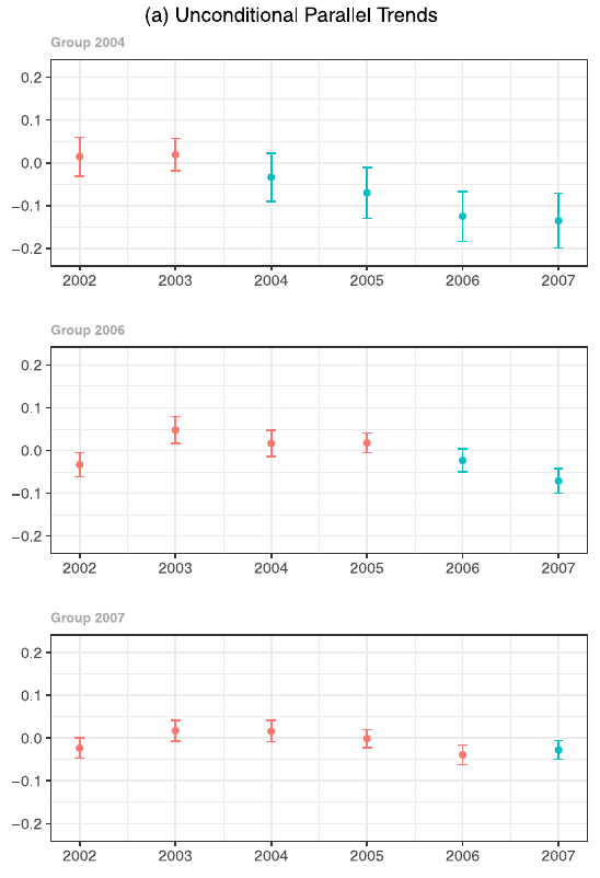
- Are untreated employment trends plausibly comparable?
- What do the pre-treatment estimates suggest?
- Minimum-wage increases differ in size. What does the binary treatment represent?
Choosing and Reporting an Estimate
- State the policy effect and population of interest.
- Identify the adoption cohorts and untreated comparisons.
- Explain parallel trends, anticipation and possible spillovers.
- Report how cohort-time effects are averaged.
- Show uncertainty and the evidence used to assess the design.
For discussion: Which of these choices would matter most if you were advising a government about another minimum-wage increase?
What We Take Forward
The basic DiD logic remains: use an untreated group’s change to construct a counterfactual.
With staggered adoption, make the comparison separately for each cohort and period, then average deliberately.
Next week: constructing a comparison for a single treated country or region using synthetic control.
References
Callaway, B., and P. H. C. Sant’Anna (2021). Difference-in-Differences with Multiple Time Periods. Journal of Econometrics, 225(2), 200–230.
Goodman-Bacon, A. (2021). Difference-in-Differences with Variation in Treatment Timing. Journal of Econometrics, 225(2), 254–277.
Sun, L., and S. Abraham (2021). Estimating Dynamic Treatment Effects in Event Studies with Heterogeneous Treatment Effects. Journal of Econometrics, 225(2), 175–199.