Weak Instruments
PP5001 · Week 5 · Martinmas 2026
Recall from the IV Lecture
We use the notation in Bound, Jaeger, and Baker: x_i is the endogenous explanatory variable, y_i is the outcome, and z_i is an excluded instrument.
x_i=\pi_0+\pi_1z_i+\nu_i,\qquad y_i=\beta_0+\beta x_i+\epsilon_i.
- Orthogonality: \operatorname{Cov}\left(z_i,\epsilon_i\right)=0.
- Relevance: \operatorname{Cov}\left(z_i,x_i\right)\ne0.
What happens when relevance is weak?
Unbiasedness and Consistency
Unbiasedness: across repeated samples of a given size, the estimator’s mean equals the true parameter.
E\left[\widehat\beta\right]=\beta.
Consistency: as the sample grows, the sampling distribution concentrates around the true parameter.
An estimator can be biased in finite samples and consistent.
Unbiasedness and Consistency: Graphically
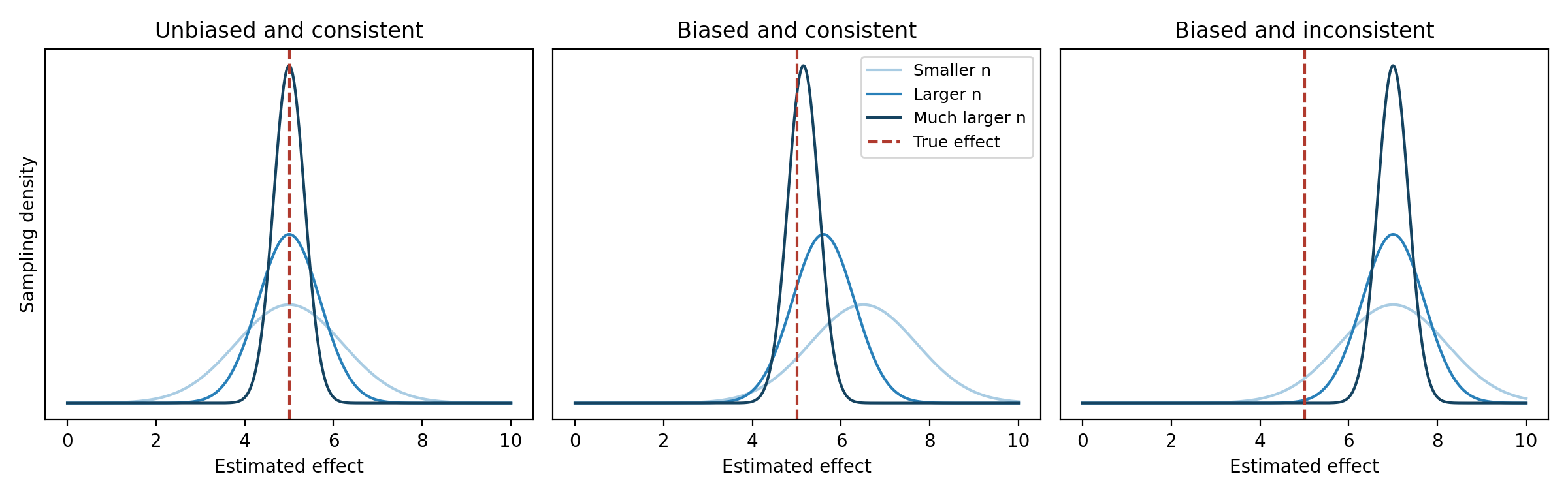
Schematic sampling distributions. Same scales in all panels. Dashed line: true effect.
The probability limit is the value that the estimate approaches as the sample size grows: the probability that the estimate differs from that value by more than any fixed positive amount goes to zero.
We write \operatorname{plim}\widehat\beta=b. An estimator is consistent if its probability limit equals the true parameter, b=\beta.
What More Observations Can Do
As the sample size increases, the OLS estimate becomes more precise, but omitted-variable bias remains. We can therefore obtain a very precise estimate of the wrong population parameter.
With valid, relevant instruments, IV can concentrate around the true effect even though its finite-sample distribution is biased.
More observations help when the identifying information is present.
The distinction concerns the sampling distribution of the coefficient itself.
The Issue
We have assumed the excluded instruments predict x_i.
For a binary instrument,
\widehat\beta^{IV}=\frac{\overline y_{z=1}-\overline y_{z=0}}{\overline x_{z=1}-\overline x_{z=0}}.
What happens when the denominator is small relative to its sampling variation?
Preliminaries: OLS
Start with y_i=\beta_0+\beta x_i+\epsilon_i. Substituting into the OLS formula gives
\widehat\beta_{OLS}=\beta+ \frac{\frac{1}{n}\sum_i\left(x_i-\bar x\right)\epsilon_i} {\frac{1}{n}\sum_i\left(x_i-\bar x\right)^2}.
As the sample grows, the sample covariance and variance converge to their population counterparts:
\operatorname{plim}\widehat\beta_{OLS}=\beta+ \frac{\sigma_{x,\epsilon}}{\sigma_x^2}.
Here \sigma_{x,\epsilon}=\operatorname{Cov}\left(x_i,\epsilon_i\right) and \sigma_x^2=\operatorname{Var}\left(x_i\right).
Preliminaries: IV
Let \widehat x_i be the first-stage fitted value. With an intercept, \overline{\widehat x}=\bar x and the first-stage residual is orthogonal to \widehat x_i.
\widehat\beta_{IV} =\frac{\sum_i\left(\widehat x_i-\bar x\right)y_i} {\sum_i\left(\widehat x_i-\bar x\right)x_i} =\beta+\frac{\frac{1}{n}\sum_i\left(\widehat x_i-\bar x\right)\epsilon_i} {\frac{1}{n}\sum_i\left(\widehat x_i-\bar x\right)^2}.
Therefore,
\operatorname{plim}\widehat\beta_{IV}=\beta+ \frac{\sigma_{\hat x,\epsilon}}{\sigma_{\hat x}^2}.
The population moments refer to the population first-stage fitted component.
What Does R^2 Measure?
R^2 is the proportion of the sample variation in the dependent variable explained by the regression.
In the first stage, the dependent variable is x_i. For OLS with an intercept,
R^2=\frac{\text{explained variation}}{\text{total variation}} =\frac{\sum_i\left(\widehat x_i-\bar x\right)^2}{\sum_i\left(x_i-\bar x\right)^2} =1-\frac{\sum_i\widehat\nu_i^2}{\sum_i\left(x_i-\bar x\right)^2}.
Here \widehat\nu_i=x_i-\widehat x_i. An R^2 of 0.01 means the instruments explain 1% of the variation in x_i.
The population counterpart is R^2_{x,z}=\sigma_{\hat x}^2/\sigma_x^2, the share of population variance explained by the instruments.
Relative Inconsistency of IV and OLS
Divide the two discrepancies from the true effect:
\frac{\operatorname{plim}\widehat\beta_{IV}-\beta} {\operatorname{plim}\widehat\beta_{OLS}-\beta} =\frac{\sigma_{\hat x,\epsilon}/\sigma_{\hat x}^2} {\sigma_{x,\epsilon}/\sigma_x^2} =\frac{\sigma_{\hat x,\epsilon}/\sigma_{x,\epsilon}} {\sigma_{\hat x}^2/\sigma_x^2}.
The denominator is the population first-stage R^2:
\boxed{\frac{\operatorname{plim}\widehat\beta_{IV}-\beta} {\operatorname{plim}\widehat\beta_{OLS}-\beta} =\frac{\sigma_{\hat x,\epsilon}/\sigma_{x,\epsilon}}{R^2_{x,z}}.}
A small R^2 magnifies the consequences of imperfect instrument validity.
One Instrument: Expressing the Result in Correlations
With one instrument,
\operatorname{plim}\widehat\beta_{IV}-\beta =\frac{\sigma_{z,\epsilon}}{\sigma_{z,x}} =\frac{\rho_{z,\epsilon}}{\rho_{z,x}}\frac{\sigma_\epsilon}{\sigma_x},
while
\operatorname{plim}\widehat\beta_{OLS}-\beta =\rho_{x,\epsilon}\frac{\sigma_\epsilon}{\sigma_x}.
Dividing cancels \sigma_\epsilon/\sigma_x:
\boxed{\frac{\operatorname{plim}\widehat\beta_{IV}-\beta} {\operatorname{plim}\widehat\beta_{OLS}-\beta} =\frac{\rho_{z,\epsilon}/\rho_{x,\epsilon}}{\rho_{x,z}}.}
When Can IV Be Worse Than OLS?
IV has a larger absolute inconsistency when
\left|\frac{\rho_{z,\epsilon}}{\rho_{x,\epsilon}}\right| >\left|\rho_{x,z}\right|.
An instrument can be much less correlated with the disturbance than x_i is, yet still produce a larger inconsistency if it barely predicts x_i.
We can measure the instrument’s predictive power. We must assess its validity using the institutional setting and supporting evidence.
Finite-Sample Bias: Valid Instruments
Now assume the instruments are exogenous. Recall
\widehat\beta_{IV}-\beta= \frac{\sum_i\left(\widehat x_i-\bar x\right)\epsilon_i} {\sum_i\left(\widehat x_i-\bar x\right)^2}.
Both the numerator and denominator change across repeated samples.
Population orthogonality does not make this ratio average to zero in a finite sample. The fitted values are estimated using the same observations.
IV can therefore be consistent but biased in finite samples.
Why Is the Bias Related to OLS?
Write the first stage as
x_i=\pi_0+\sum_{j=1}^{K}\pi_jz_{ji}+\nu_i.
The instruments are exogenous. Endogeneity remains in \nu_i, which is correlated with \epsilon_i.
- The first-stage regression fits some of the sample variation in \nu_i by chance.
- That fitted variation enters \widehat x_i and can be related to \epsilon_i.
- With weak instruments, this can be a substantial part of the fitted variation.
This pulls 2SLS towards OLS. Adding instruments can increase the amount of noise fitted in the first stage.
Partial R^2
Compare the first stage with the excluded instruments to the regression containing the controls alone.
\text{partial }R^2=\frac{R_U^2-R_R^2}{1-R_R^2}=\frac{SSR_R-SSR_U}{SSR_R}.
This measures the share of variation remaining after the controls that the excluded instruments explain.
The overall first-stage R^2 also reflects the controls.
First-Stage F
With three excluded instruments, test
H_0:\pi_1=\pi_2=\pi_3=0.
Report the test on the excluded instruments, together with partial R^2.
An F below 10 is a warning sign. An F above 10 does not guarantee reliable conventional IV inference.
Use a test appropriate to the assumptions about the disturbances.
Relative Bias and the First-Stage F
Deriving the finite-sample bias of IV is complicated. Interested readers can find the argument in Bound, Jaeger, and Baker (1995).
Under certain assumptions, the bias of IV relative to the bias of OLS is approximately
\frac{\operatorname{Bias}\left(\widehat\beta_{IV}\right)} {\operatorname{Bias}\left(\widehat\beta_{OLS}\right)}\approx\frac{1}{F}.
For example, F=10 suggests an IV bias roughly one-tenth of the OLS bias.
This is why we report the first-stage F alongside the IV estimate: it helps us assess how serious finite-sample bias may be.
Weak Instruments and Inference
A conventional IV t statistic can have a misleading reference distribution when instruments are weak.
Heteroskedasticity-consistent standard errors do not solve this problem.
Anderson–Rubin idea: for a proposed effect b, test whether the excluded instruments predict y_i-bx_i, accounting for the controls.
An appropriate weak-instrument-robust test remains valid when relevance is weak. Its confidence set can be very wide.
An Illustration
Retain the relationships from the earlier illustration:
x_i=1+\pi_1z_i+2w_i+\nu_i, y_i=2+5x_i+20w_i+e_i.
w_i is omitted from the estimated earnings equation. The true effect is 5.
z_i is binary and independent of w_i, \nu_i and e_i.
Strong first stage: \pi_1=5. No population first stage: \pi_1=0.
Wald Estimator with Strong Instruments
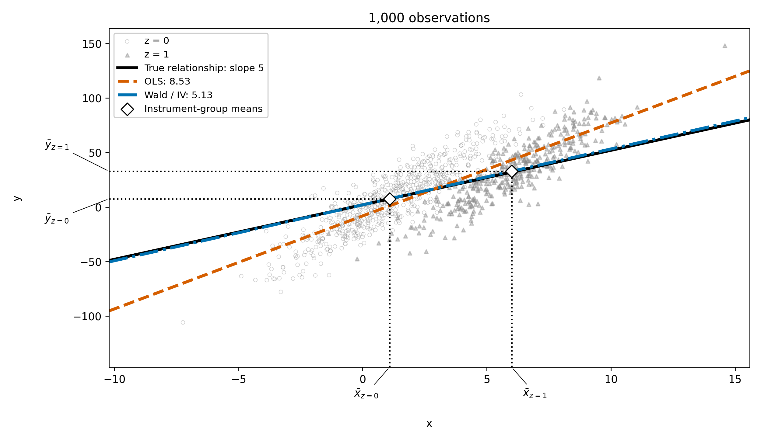
1,000 observations. The diamonds mark the two instrument-group means.
Strong Instruments: Results
| Statistic | Value |
|---|---|
| OLS slope | 8.532 |
| IV slope | 5.126 |
| Reported IV standard error | 0.276 |
| First-stage coefficient | 4.914 |
| First-stage F | 1,261.87 |
The IV estimate is close to the true effect of 5.
Wald Estimator with No First Stage
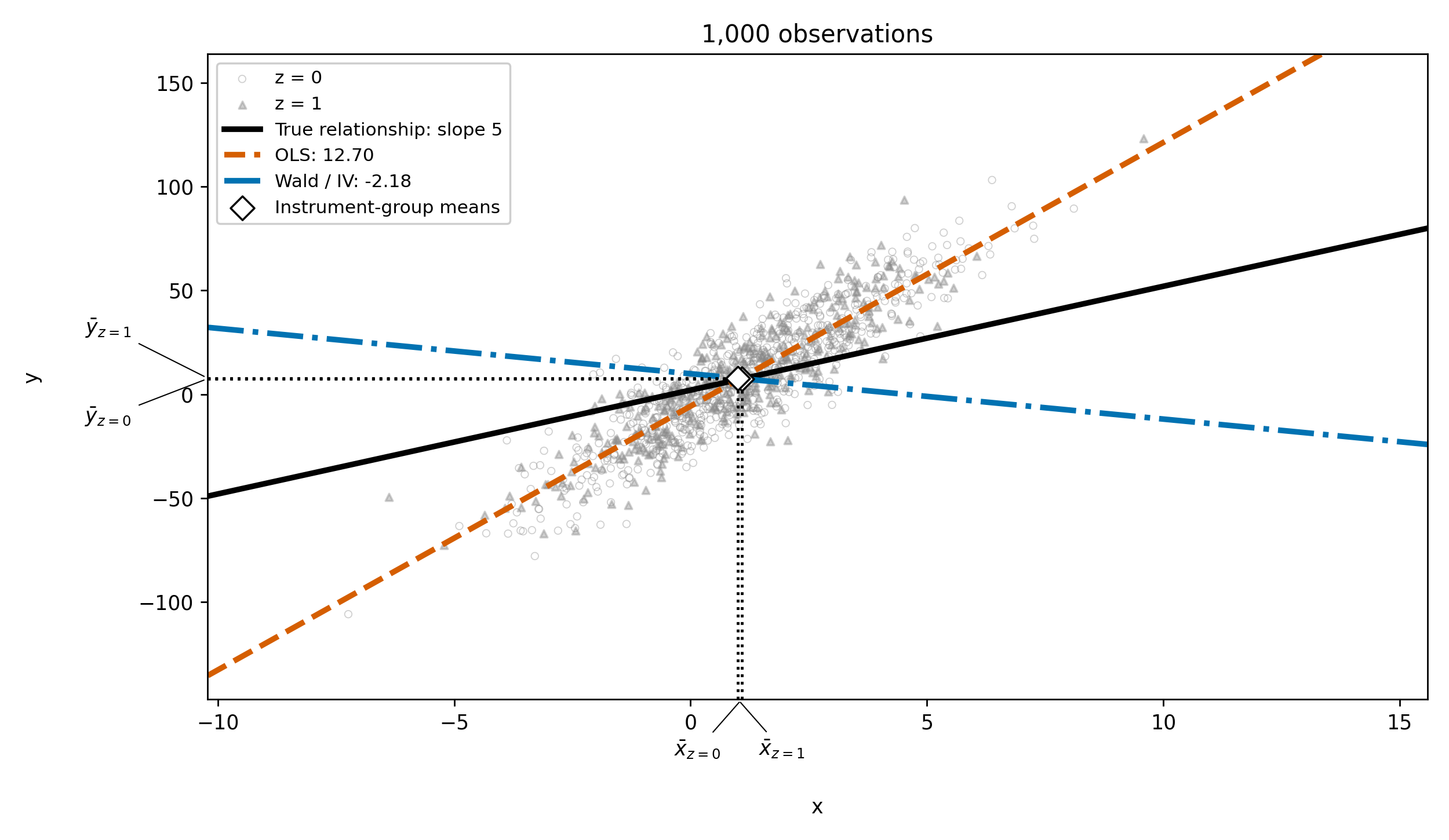
1,000 observations. Population first-stage coefficient is zero.
No First Stage: 1,000 Observations
| Statistic | Value |
|---|---|
| OLS slope | 12.701 |
| IV slope | −2.185 |
| Reported IV standard error | 25.781 |
| First-stage coefficient | −0.086 |
| First-stage F | 0.39 |
The two instrument groups have almost the same mean x_i.
No First Stage, but Many Observations
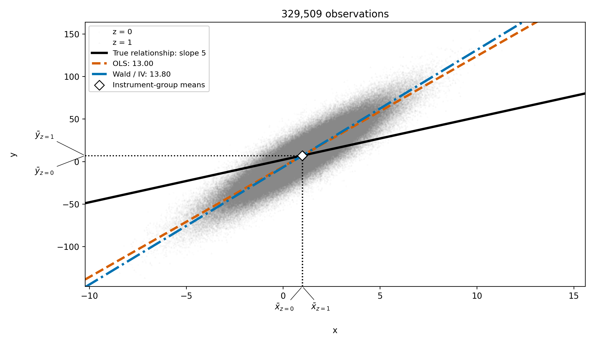
All 329,509 observations are displayed. Dotted lines project the group means onto both axes.
The Second Stage Looks Reassuring
| Statistic | Value |
|---|---|
| Observations | 329,509 |
| OLS slope | 12.997 |
| IV slope | 13.798 |
| Reported IV standard error | 4.265 |
The true effect is 5.
Would anything in these second-stage results alert you to a problem?
Look at the First Stage
| Statistic | Value |
|---|---|
| First-stage coefficient | −0.0113 |
| First-stage F | 2.02 |
| First-stage R^2 | approximately 0.000006 |
The population first stage is zero. A large sample cannot create relevance.
This illustrative draw shows that IV can resemble OLS. Other draws can give very different IV estimates.
Angrist and Krueger: Data
For discussion
Describe the Census data, the samples and birth cohorts used in the paper, and the sample of 329,509 men used in our exercise.
Explain how schooling, earnings and quarter of birth are measured.
Who is included in the analysis, and how might that affect the population to which the results apply?
Angrist and Krueger: Identification Strategy
For discussion
State the causal question and identify the outcome, endogenous explanatory variable and instruments.
Explain how school-entry and compulsory-schooling laws generate variation in schooling.
Discuss relevance, independence and exclusion, and the monotonicity assumption needed for a local causal interpretation.
Whose schooling is affected?
Give a plausible threat to the assumptions.
Angrist and Krueger’s Natural Experiment

Angrist and Krueger’s Framework
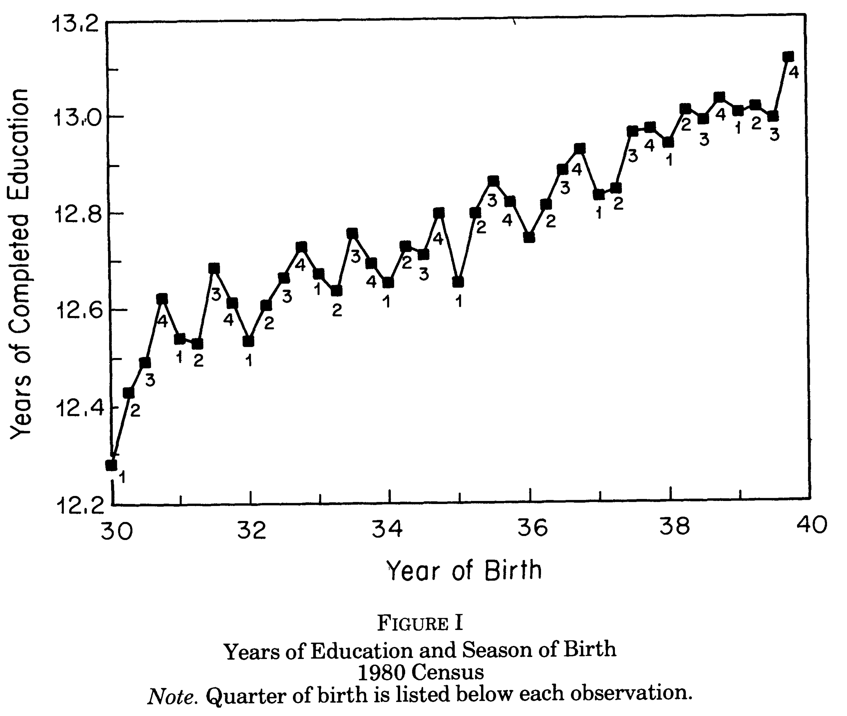
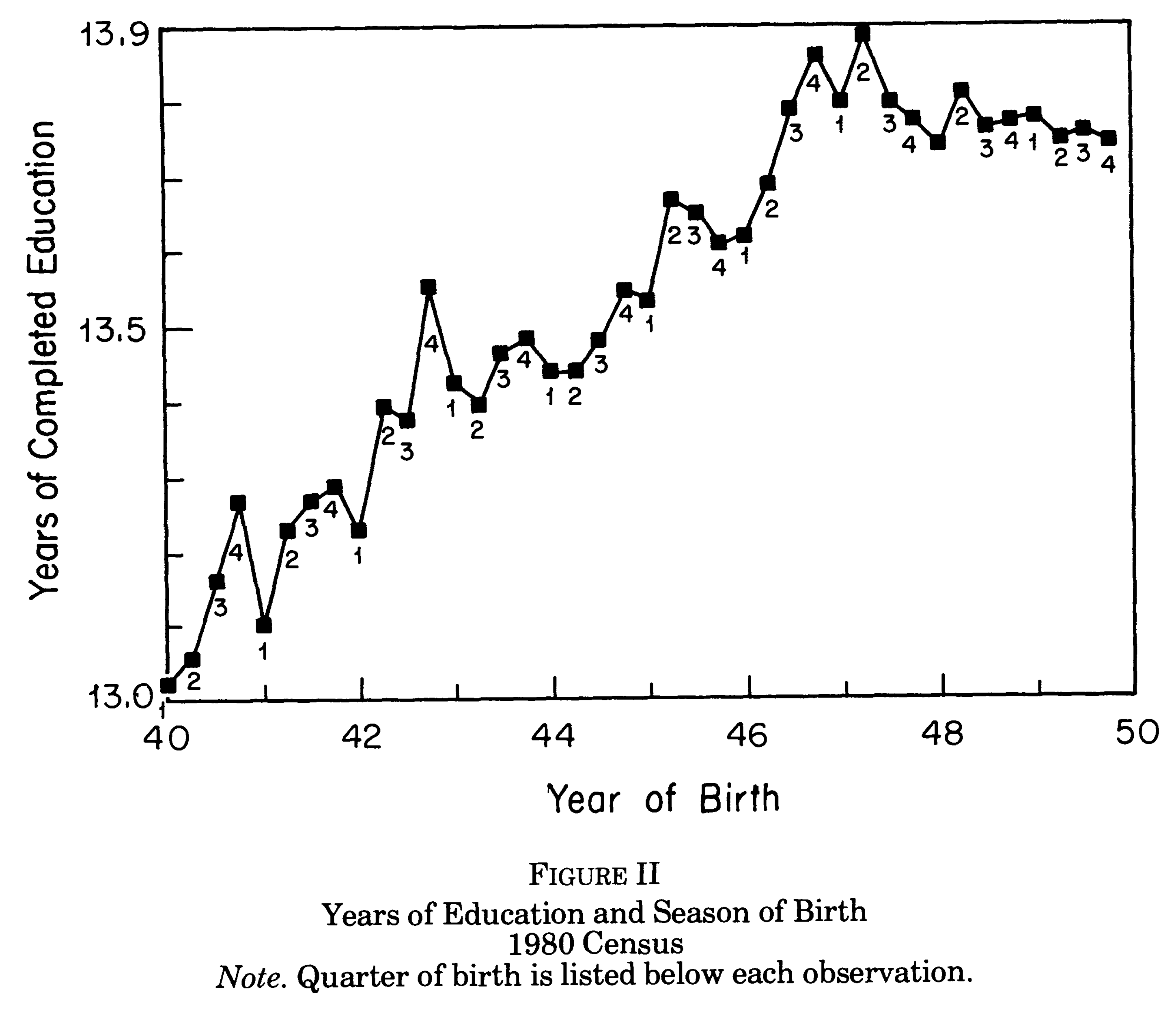
School-entry and compulsory-schooling laws create a relationship between quarter of birth and schooling.
- Outcome: log weekly earnings.
- Endogenous explanatory variable: years of schooling.
- Excluded instruments: quarter-of-birth indicators, and in larger specifications interactions with year of birth.
- Controls: demographic characteristics, region and age or year of birth.
1980 Census sample: 329,509 men born in 1930–1939.
Angrist–Krueger: Figure I
For discussion
Angrist and Krueger (1991).
Angrist–Krueger: Figure II
For discussion
Angrist and Krueger (1991).
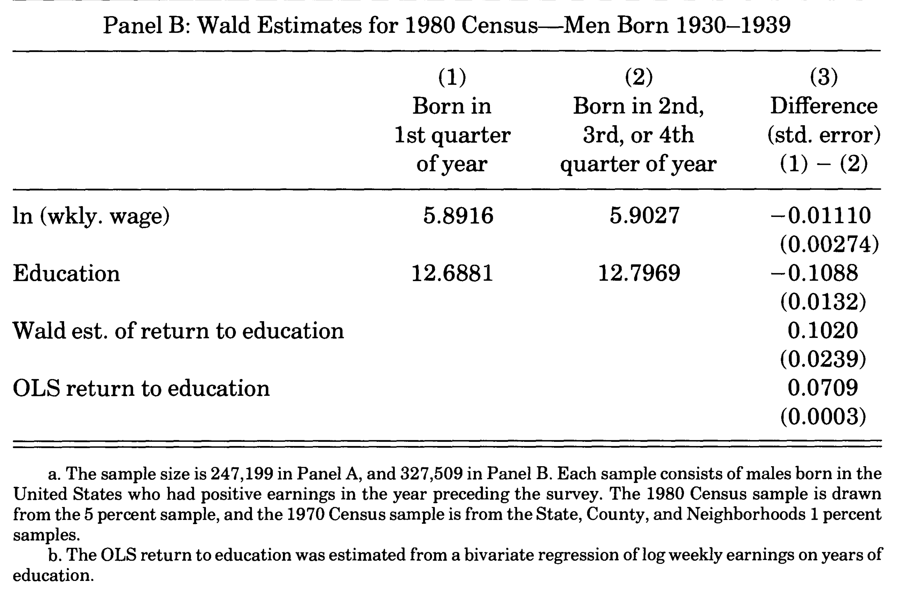
Angrist–Krueger: Table III, Panel B
For discussion
Angrist and Krueger (1991).
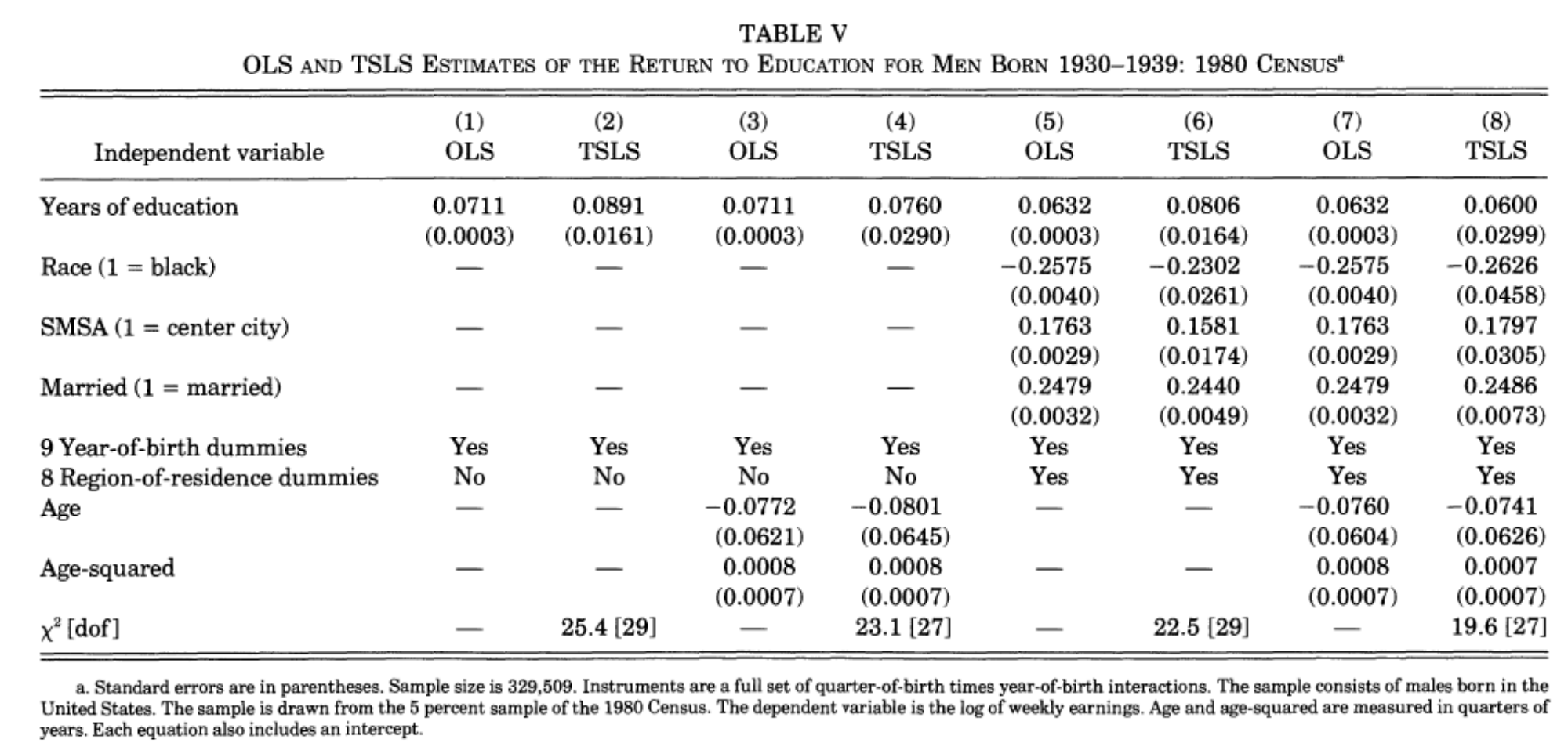
Angrist–Krueger: Table V
For discussion
Angrist and Krueger (1991).
Angrist–Krueger: Table VII
For discussion
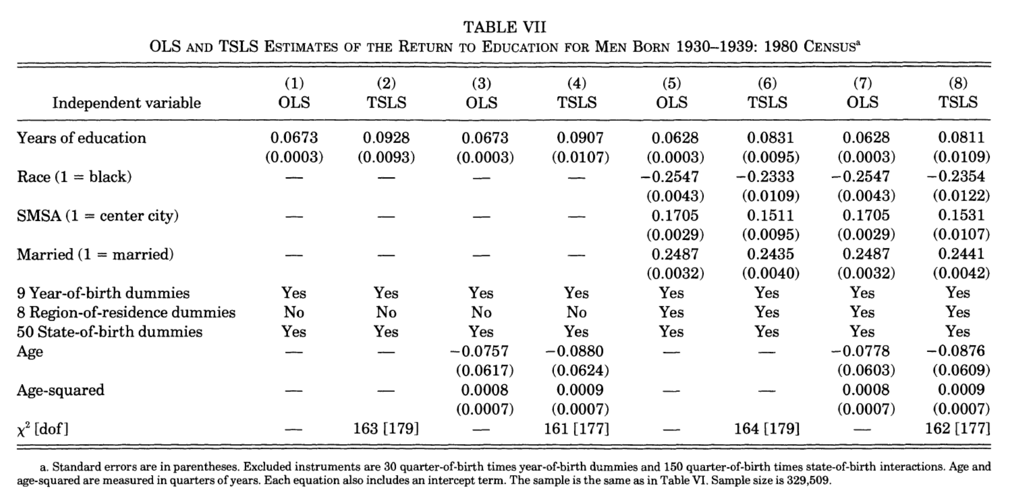
Angrist and Krueger (1991).
Bound, Jaeger, and Baker: What Is the Problem?
For discussion
Why might an IV estimate close to OLS be misleading when the instruments are weak?
What first-stage evidence would help you judge the estimates?
Explain the concern that Bound, Jaeger, and Baker raise about the Angrist–Krueger analysis.
Bound–Jaeger–Baker: Table 1
For discussion
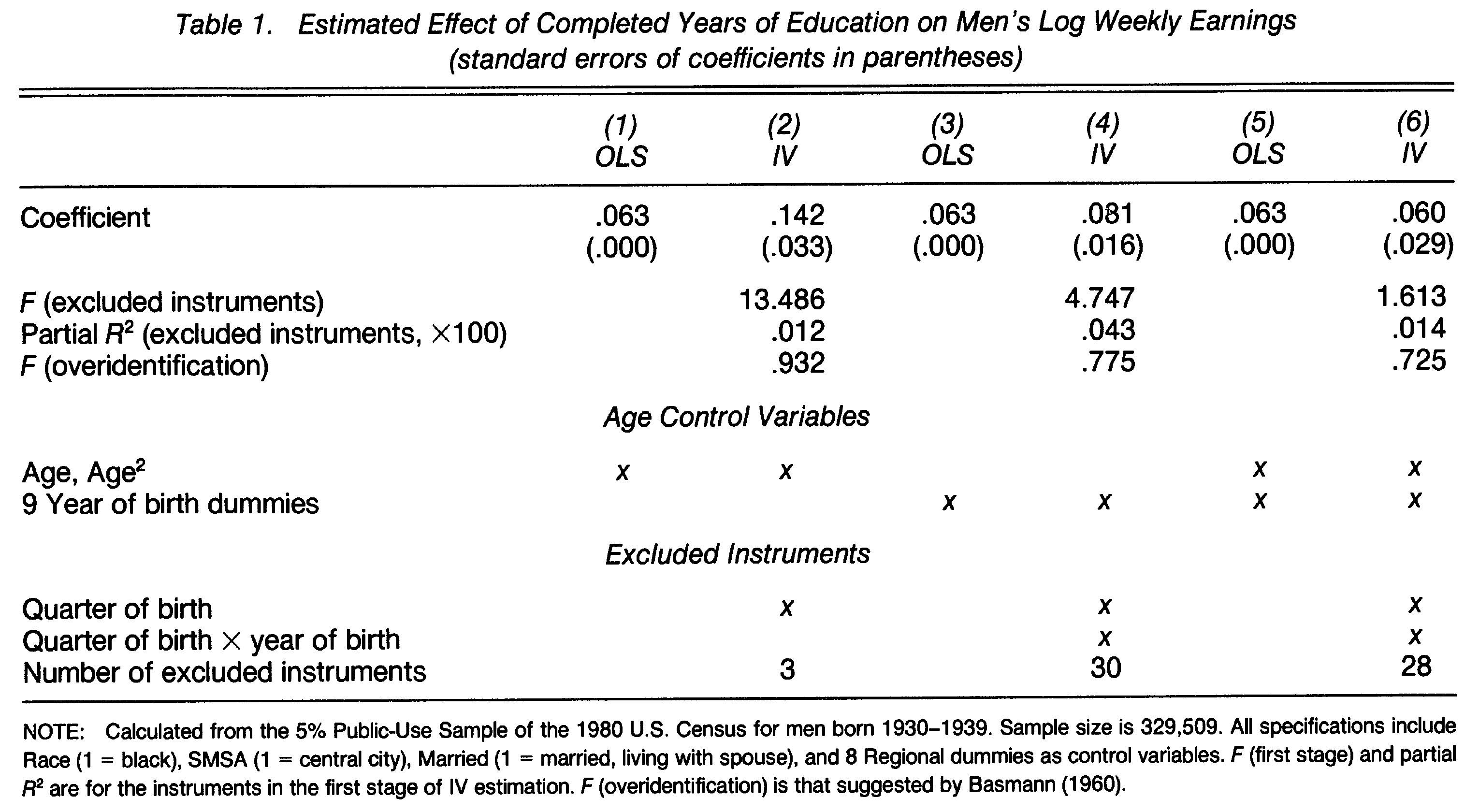
Bound, Jaeger, and Baker (1995).
Bound–Jaeger–Baker: Table 2
For discussion
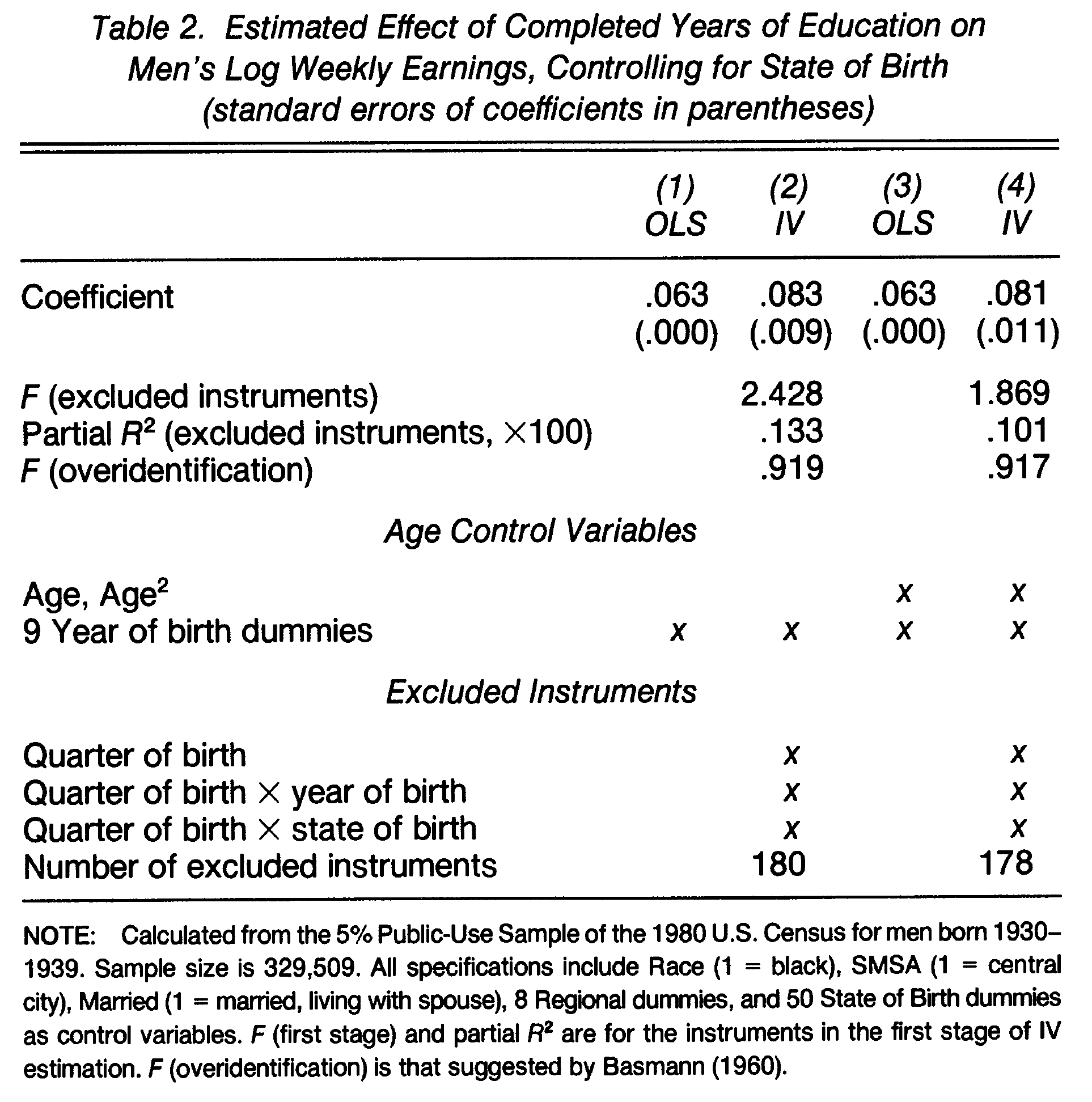
Bound, Jaeger, and Baker (1995).
Bound–Jaeger–Baker: Table 3
For discussion
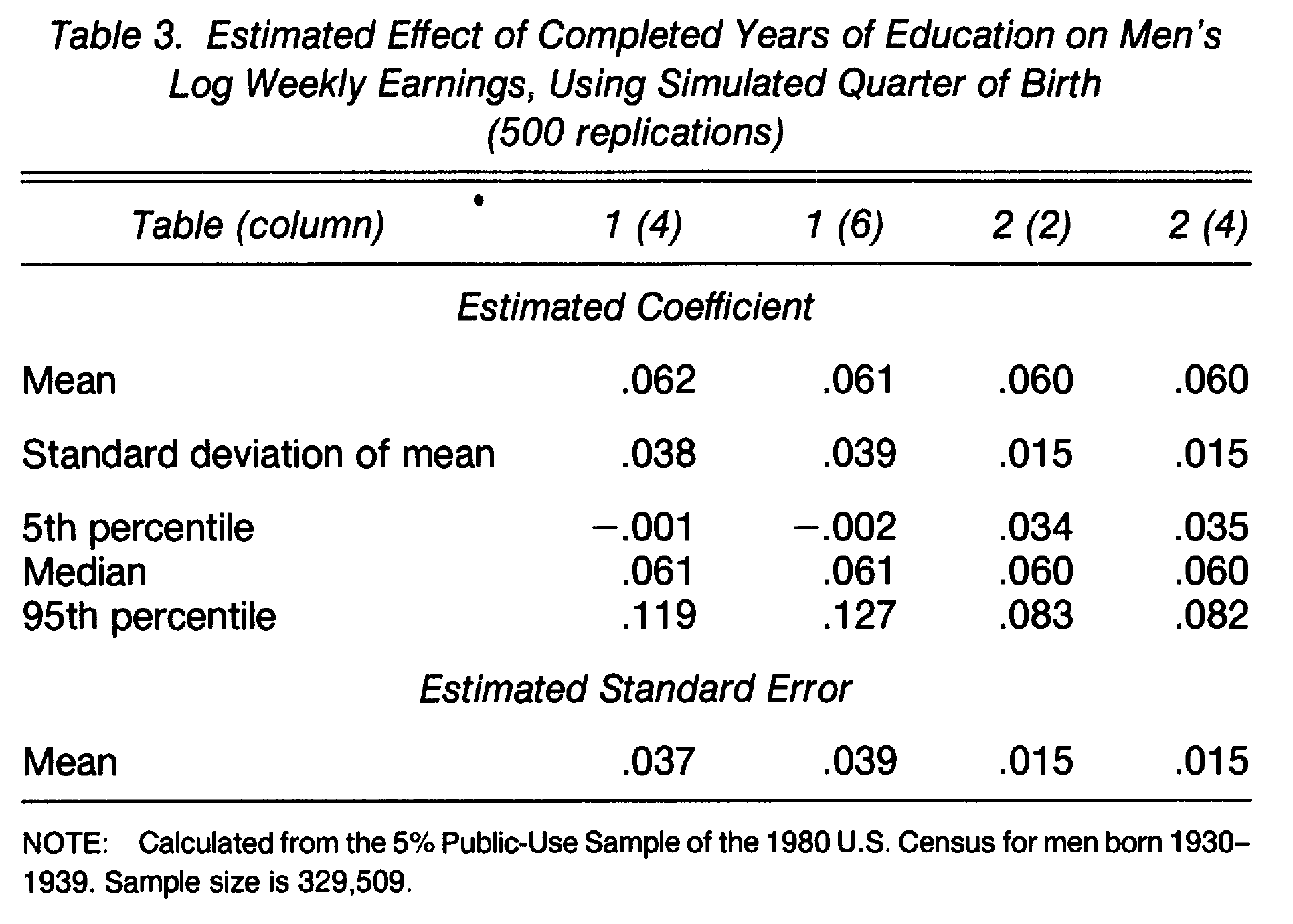
Bound, Jaeger, and Baker (1995).
Does Schooling Alone Explain the Earnings Pattern?
For discussion
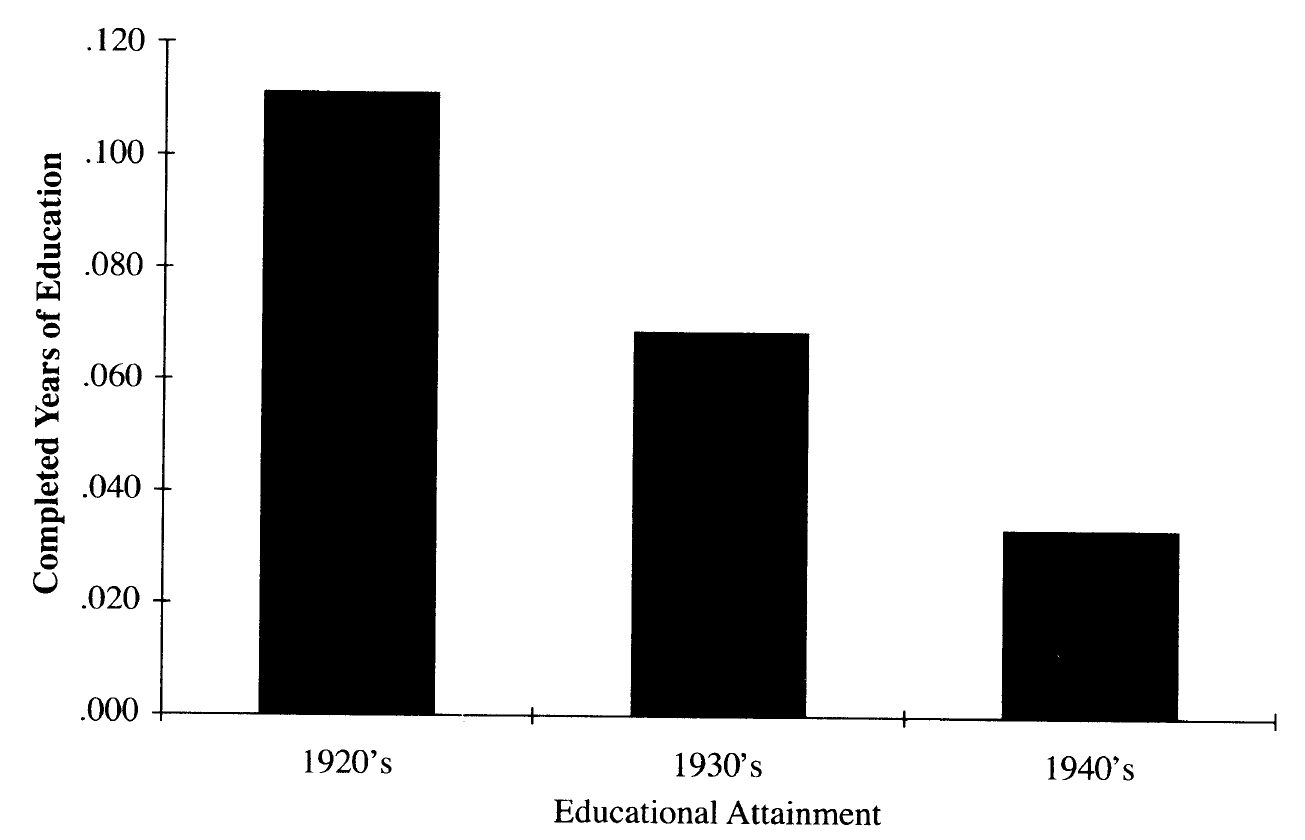
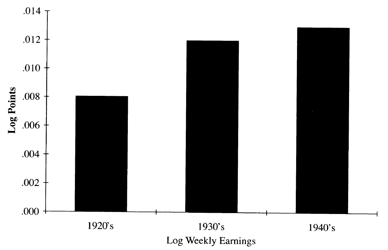
Figure 1. Third-quarter minus first-quarter differences in educational attainment and log weekly earnings, by birth decade. Source: Bound and Jaeger (2000), Table 2.
What Should We Take Away?
The story behind an instrument matters. Weak relevance makes small failures of validity especially consequential.
Second-stage estimates and reported standard errors are insufficient to assess the design.
Report first-stage coefficients, the excluded-instrument F and partial R^2 alongside IV results.
For quarter of birth, investigate both relevance and exclusion.
Problem Set 2
- Calculate AK’s Wald estimate directly from the sample means.
- Reproduce it using IV on the same sample.
- Use three quarter-of-birth indicators as excluded instruments.
- Change the controls, particularly age and age squared.
- Present the first-stage results alongside IV.
Due: Friday 30 October, 12 noon (Week 7).
References
- Angrist, J. D., and A. B. Krueger (1991). “Does Compulsory School Attendance Affect Schooling and Earnings?” Quarterly Journal of Economics 106(4): 979–1014. Paper.
- Bound, J., D. A. Jaeger, and R. M. Baker (1995). “Problems with Instrumental Variables Estimation When the Correlation Between the Instruments and the Endogenous Explanatory Variable Is Weak.” Journal of the American Statistical Association 90(430): 443–450. Paper.
- Bound, J., and D. A. Jaeger (2000). “Do Compulsory School Attendance Laws Alone Explain the Association between Earnings and Quarter of Birth?” Research in Labor Economics 19: 83–108. Paper.
- Staiger, D., and J. H. Stock (1997). “Instrumental Variables Regression with Weak Instruments.” Econometrica 65(3): 557–586. Paper.