Selection Bias and Experiments

PP5001 · Week 1

Professor David A. Jaeger

The Research Question

All research should start with a question to be answered. We are interested in causal relationships: how does a policy or programme affect an outcome?

Does university attendance raise subsequent earnings? The counterfactual is: what would those who attended university have earned had they not attended?

We begin with the DAGs from PP5000, then connect the confounding problem to regression, potential outcomes, and random assignment.

Causal Diagrams and the Comparison Group

flowchart LR
    A["Ability: A"] --> D["University attendance: D"]
    A --> Y["Later earnings: Y"]
    D --> Y

The arrow \(D\to Y\) is the effect we want to estimate. The backdoor path \(D\leftarrow A\to Y\) gives another reason those who attend university and those who do not might have different earnings.

Conditioning on \(A\) blocks this path if this diagram adequately represents the confounding. The arrows express assumptions, not conclusions from a correlation matrix.

Not Every Control Is a Good Control

The causal role of a variable determines whether conditioning on it helps answer our question.

• Confounder: \(D\leftarrow A\to Y\). Conditioning on \(A\) blocks this backdoor path.
• Mediator: \(D\to M\to Y\). Conditioning on \(M\) removes part of the pathway through which treatment operates; we are no longer estimating the total effect in the same way.
• Collider: \(D\to C\leftarrow U\to Y\). Conditioning on \(C\) opens a previously blocked path.

Ability measured before university and occupation after university can therefore play very different roles in an earnings regression.

Omitted Variables Bias (1): The Model

To make the importance of confounding concrete, suppose the earnings equation is

\[Y_i=\beta_0+\beta_1 D_i+\beta_2 A_i+\varepsilon_i, \qquad E[\varepsilon_i\mid D_i,A_i]=0.\]

\(D_i=1\) indicates university attendance, and \(D_i=0\) no university attendance. \(A_i\) denotes ability before university. For this illustration, \(\beta_1\) is the same causal effect for everyone.

In practice, relevant characteristics may be difficult to measure. If we leave out \(A_i\), it becomes part of the disturbance:

\[Y_i=\beta_0+\beta_1 D_i+u_i,\qquad u_i=\beta_2 A_i+\varepsilon_i.\]

The issue is whether this new disturbance is associated with university attendance.

DGP Parameters and Estimated Coefficients

The true population relationship is

\[Y_i=\beta_0+\beta_1D_i+\beta_2A_i+\varepsilon_i.\]

If ability is observed, the fitted full regression is

\[\widehat Y_i=\widehat\beta_0+\widehat\beta_1D_i+\widehat\beta_2A_i.\]

If we omit ability, we fit a different, short regression:

\[\widehat Y_i^{S}=\widehat\beta_0^{S}+\widehat\beta_1^{S}D_i.\]

Hats denote sample estimates. The superscript \(S\) means short regression; its population slope \(\beta_1^{S}\) need not equal the causal effect \(\beta_1\).

Omitted Variables Bias (2): Recall the OLS Slope

The slope in the sample regression of \(Y\) on an intercept and \(D\) is

\[\widehat\beta_1^{S}= \frac{\sum_i(D_i-\overline D)(Y_i-\overline Y)} {\sum_i(D_i-\overline D)^2}.\]

Its population counterpart is

\[\beta_1^{S}=\frac{\operatorname{Cov}(D_i,Y_i)}{\operatorname{Var}(D_i)}.\]

We use the population expression to see what the short regression identifies. The coefficient is \(\beta_1^{S}\); we must establish when it equals the causal parameter \(\beta_1\).

Omitted Variables Bias (3): Substitute and Expand

Substitute the full earnings equation into the covariance:

\[\begin{aligned} \beta_1^{S} &=\frac{\operatorname{Cov}(D_i,\beta_0+\beta_1 D_i+\beta_2 A_i+\varepsilon_i)} {\operatorname{Var}(D_i)}\\[4pt] &=\frac{\beta_1\operatorname{Var}(D_i)+\beta_2\operatorname{Cov}(D_i,A_i) +\operatorname{Cov}(D_i,\varepsilon_i)}{\operatorname{Var}(D_i)}\\[4pt] &=\beta_1+\beta_2\frac{\operatorname{Cov}(D_i,A_i)}{\operatorname{Var}(D_i)}. \end{aligned}\]

The intercept is constant, so its covariance with \(D_i\) is zero. The conditional-mean assumption implies \(\operatorname{Cov}(D_i,\varepsilon_i)=0\).

Neither step eliminates the covariance between \(D_i\) and the omitted \(A_i\).

Omitted Variables Bias (4): Regress Ability on Attendance

Write the population regression of \(A_i\) on \(D_i\) as

\[A_i=\gamma_0+\gamma_1D_i+v_i, \qquad E[v_i]=0,\quad\operatorname{Cov}(D_i,v_i)=0.\]

If ability is observed, its sample regression is

\[A_i=\widehat\gamma_0+\widehat\gamma_1D_i+\widehat v_i, \qquad \widehat A_i=\widehat\gamma_0+\widehat\gamma_1D_i.\]

Because \(D\) is binary,

\[\gamma_1=E[A_i\mid D_i=1]-E[A_i\mid D_i=0], \qquad \widehat\gamma_1=\overline A_{D=1}-\overline A_{D=0}.\]

This describes the ability difference between groups. It does not say that university attendance causes pre-existing ability.

Omitted Variables Bias (4): Substitute the Auxiliary Regression

Substitute \(A_i=\gamma_0+\gamma_1D_i+v_i\) into the earnings DGP:

\[\begin{aligned} Y_i&=\beta_0+\beta_1D_i+\beta_2(\gamma_0+\gamma_1D_i+v_i)+\varepsilon_i\\[4pt] &=(\beta_0+\beta_2\gamma_0)+(\beta_1+\beta_2\gamma_1)D_i +(\beta_2v_i+\varepsilon_i). \end{aligned}\]

The last term is uncorrelated with \(D_i\). Hence the population short regression has

\[\beta_0^{S}=\beta_0+\beta_2\gamma_0, \qquad \boxed{\beta_1^{S}=\beta_1+\beta_2\gamma_1}.\]

The bias is the effect of ability on earnings, multiplied by the ability difference between those who attend university and those who do not.

Omitted Variables Bias (5): When and in Which Direction?

\[\beta_1^{S}-\beta_1=\beta_2\gamma_1.\]

With one omitted variable, bias requires both that \(A\) predicts the outcome (\(\beta_2\ne0\)) and that \(A\) is associated with university attendance (\(\gamma_1\ne0\)).

Suppose ability raises earnings and those who attend university have higher ability on average. Then \(\beta_2>0\) and \(\gamma_1>0\): the short regression overstates the effect of university attendance.

For an illustrative calculation, if \(\beta_1=1000\), \(\beta_2=200\), and \(\gamma_1=2\), then

\[\beta_1^{S}=1000+200(2)=1400.\]

These are hypothetical numbers. The DAG does not establish the signs or magnitudes by itself.

Omitted Variables Bias (6): A Binary Treatment

Write \(p=P(D=1)\), where \(0<p<1\). Because \(D\) is binary,

\[\begin{aligned} E[DA]&=pE[A\mid D=1],\\ E[A]&=pE[A\mid D=1]+(1-p)E[A\mid D=0],\\ \operatorname{Cov}(D,A) &=p(1-p)\left(E[A\mid D=1]-E[A\mid D=0]\right). \end{aligned}\]

Dividing by \(\operatorname{Var}(D)=p(1-p)\) gives

\[\boxed{\beta_1^{S}=\beta_1+\beta_2\left(E[A\mid D=1]-E[A\mid D=0]\right).}\]

The auxiliary-regression slope is simply the baseline difference in means.

Potential Outcomes: A Short Review

Consider one individual, \(i\). Ideally, we would observe earnings in both states of the world:

\[\begin{aligned} Y_i^1 &: \text{ earnings with university attendance},\\ Y_i^0 &: \text{ earnings without university attendance}. \end{aligned}\]

Only one is observed. For \(D_i\in\{0,1\}\),

\[\begin{aligned} Y_i&=D_iY_i^1+(1-D_i)Y_i^0\\ &=Y_i^0+(Y_i^1-Y_i^0)D_i. \end{aligned}\]

The missing potential outcome is the counterfactual. We keep the superscript notation from PP5000; the treatment state is not an exponent.

Treatment Effect: Deriving the Decomposition

The observed population difference is

\[\begin{aligned} &E[Y_i\mid D_i=1]-E[Y_i\mid D_i=0]\\ &=E[Y_i^1\mid D_i=1]-E[Y_i^0\mid D_i=0]\\ &=E[Y_i^1\mid D_i=1]-E[Y_i^0\mid D_i=1]\\ &\quad+E[Y_i^0\mid D_i=1]-E[Y_i^0\mid D_i=0]. \end{aligned}\]

We have added and subtracted the untreated potential outcome of the treated group. That is precisely the counterfactual we cannot observe directly.

Effect of Treatment on the Treated and Selection Bias

\[\underbrace{E[Y_i^1-Y_i^0\mid D_i=1]}_{\text{average treatment effect on the treated: ATT}}\]

How did university attendance affect those who attended, relative to what those same people would have earned without attending?

\[\underbrace{E[Y_i^0\mid D_i=1]-E[Y_i^0\mid D_i=0]}_{\text{selection bias}}\]

Would those who attended university and those who did not have had different earnings even without university attendance? The observed difference equals ATT plus this term. Neither identity requires constant treatment effects.

Regression Analysis and Experiments (1)

For now, assume that the treatment effect is the same for everyone: \(Y_i^1-Y_i^0=\beta_1\).

Starting from the observed-outcome identity, write

\[\begin{aligned} Y_i&=Y_i^0+\beta_1 D_i\\ &=\underbrace{E[Y_i^0]}_{\mu_0}+\beta_1 D_i +\underbrace{\left(Y_i^0-E[Y_i^0]\right)}_{\eta_i}. \end{aligned}\]

The regression disturbance is the part of untreated potential earnings that differs from its population mean. Although \(E[\eta_i]=0\), it need not be true that \(E[\eta_i\mid D_i]=0\).

Retains the construction in the original Regression Analysis and Experiments (1). The intercept is \(\mu_0=E[Y_i^0]=\beta_0+\beta_2E[A_i]\), which differs from \(\beta_0\) in the full earnings model.

Regression Analysis and Experiments (2)

Taking conditional expectations in the two groups gives

\[\begin{aligned} E[Y_i\mid D_i=1]&=\mu_0+\beta_1+E[\eta_i\mid D_i=1],\\ E[Y_i\mid D_i=0]&=\mu_0+E[\eta_i\mid D_i=0]. \end{aligned}\]

Subtracting,

\[\begin{aligned} &E[Y_i\mid D_i=1]-E[Y_i\mid D_i=0]\\ &=\beta_1+\underbrace{E[\eta_i\mid D_i=1]-E[\eta_i\mid D_i=0]}_{\text{selection bias}}. \end{aligned}\]

A regression comparison is contaminated when the disturbance has different means across the two groups.

Regression Analysis and Experiments (3): Back to OVB

In our full model, \(Y_i^0=\beta_0+\beta_2 A_i+\varepsilon_i\), so

\[\eta_i=\beta_2\left(A_i-E[A_i]\right)+\varepsilon_i.\]

Consequently,

\[\begin{aligned} &E[\eta_i\mid D_i=1]-E[\eta_i\mid D_i=0]\\ &=E[Y_i^0\mid D_i=1]-E[Y_i^0\mid D_i=0]\\ &=\beta_2\left(E[A_i\mid D_i=1]-E[A_i\mid D_i=0]\right) =\beta_2\gamma_1. \end{aligned}\]

The OVB term and selection bias are the same quantity in this model. The DAG, regression, and potential outcomes describe the same problem.

Random Assignment and Selection Bias

If treatment is independent of both potential outcomes, then

\[E[Y_i^0\mid D_i=1]=E[Y_i^0\mid D_i=0].\]

We can therefore write

\[\begin{aligned} E[Y_i\mid D_i=1]-E[Y_i\mid D_i=0] &=E[Y_i^1\mid D_i=1]-E[Y_i^0\mid D_i=1]\\ &=\underbrace{E[Y_i^1-Y_i^0\mid D_i=1]}_{\text{ATT}}\\[6pt] &=\underbrace{E[Y_i^1-Y_i^0]}_{\text{ATE}}. \end{aligned}\]

The first equality removes selection bias. The last uses independence of treatment and the treatment effect. Under random assignment, ATT and ATE coincide in the population.

The Importance of Random Assignment

As a thought experiment, suppose university attendance itself could be randomly assigned.

flowchart LR
    A["Ability"] --> Y["Later earnings"]
    R["Random assignment"] --> D["University attendance"]
    D --> Y

The untreated group supplies an appropriate counterfactual in expectation over assignment. It represents what would have happened to the treatment group without treatment.

\[\widehat\beta_1^{S}=\overline Y_{D=1}-\overline Y_{D=0}.\]

Under random assignment, \(\beta_1^{S}=\beta_1\) in the constant-effect model. The estimated short and full regressions can still differ in a finite sample.

Randomisation does not guarantee identical realised groups or eliminate uncertainty. It also does not make the experimental sample representative of a wider population.

A Taxonomy of Experiments

Not all experiments are the same. Following Harrison and List (2004), distinguish:

• Lab experiment: a conventional subject pool, an abstract task, and substantial experimental control.
• Artefactual field experiment: a lab experiment with a non-standard subject pool, such as actual traders rather than undergraduates.
• Framed field experiment: real context, task, and stakes; subjects know they are in an experiment.
• Natural field experiment: people act in their ordinary setting without knowing they are being studied.

These designs offer different combinations of control and context. A field setting does not by itself establish external validity; we still need to ask to whom and to what setting the result applies.

Designing an Experiment

Start with the policy question and the outcomes through which we will assess it.

• Treatment: what is the policy question, what is offered, and to whom?
• Unit of randomisation: individuals, schools, villages, or another unit? Assignment and possible spillovers must be considered together.
• Outcomes and effect sizes: what will we measure, when, and what effect would matter for policy?
• Subgroups: do we want to detect different effects for particular groups? Plan those comparisons and their precision in advance.

These decisions inform the pre-analysis plan. Power calculations then establish the sample size needed for the planned comparisons.

Randomisation: Simple, Stratified, and Blocked

Simple random assignment leaves baseline balance to chance in any one sample.

Stratified or blocked assignment randomises within groups defined before treatment—for example, region or baseline attainment. Fixing treatment numbers within blocks controls their representation in each arm and can improve precision.

This does not guarantee exact balance on every characteristic. Analysis should respect the assignment design, especially if treatment probabilities differ between blocks.

Adjusting for region afterwards is not evidence that randomisation was blocked by region. We must read how assignment was actually implemented.

Registration and Pre-Analysis Plans

Registering an experiment records its design before the results are known. A pre-analysis plan specifies the primary outcomes, regressions, subgroup comparisons, sample size and its justification, and other analysis choices in advance.

With many outcomes and specifications, researchers have considerable scope to find a significant result by chance. A plan helps the reader distinguish an anticipated test from a result found through searching.

Prespecification does not prevent every difficulty in implementation. Changes should be explained, dated where possible, and assessed alongside the original analysis and robustness checks.

The sample-size justification connects the plan to power: how many observations do we need to detect an effect of policy interest? Record the calculation and its assumptions in the plan.

Statistical Power

\[\text{Power}=P(\text{reject }H_0\mid\text{specified alternative is true})=1-\beta.\]

Power is the probability of avoiding a Type II error. Put another way, it is the probability of landing in the rejection region when the effect takes the specified nonzero value.

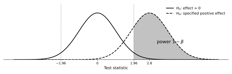
The same rejection rule can have high power against a large effect and low power against a small one. A non-significant result must be read alongside the precision of the estimate.

From Power to the Minimum Detectable Effect

In planning a study, we can fix the desired power and ask what effect we could detect. With independent observations and a common outcome variance \(\sigma^2\), the usual normal approximation gives

\[\mathrm{MDE}=\left(z_{1-\alpha/2}+z_{1-\beta}\right) \sqrt{\frac{\sigma^2}{n_T}+\frac{\sigma^2}{n_C}}.\]

• Lower outcome variance makes small effects easier to detect. Predictive baseline controls can help here.
• Larger samples shrink the standard error and lower the MDE.
• Requiring greater power, or a more stringent significance level, raises the MDE for a fixed sample.

The MDE is a feature of a design and a chosen testing standard—not the smallest effect that could ever produce a significant estimate.

Power Formula and a Worked Example

Assume equal variances \(\sigma^2\), equal arms of size \(n\), and a two-sided test at level \(\alpha\). Rearranging the MDE expression to detect an effect \(\Delta\) with power \(1-\beta\) gives

\[n=2\left(z_{1-\alpha/2}+z_{1-\beta}\right)^2\frac{\sigma^2}{\Delta^2}.\]

Take \(\sigma=4\), \(\Delta=0.2\) standard deviations (\(=0.8\)), \(\alpha=0.05\), and power \(0.80\). Using \(z_{0.975}\simeq1.96\) and \(z_{0.80}\simeq0.84\),

\[n=2(1.96+0.84)^2\frac{16}{0.64}\simeq392\quad\text{per arm}.\]

Raising power to \(0.90\) (\(z_{0.90}\simeq1.28\)) gives roughly 525 per arm. Holding the target effect at 0.8 and halving the standard deviation to 2 gives roughly 98 per arm at 80% power.

This is the worked example in the original experiments deck, with the same numbers. These are normal-approximation calculations using rounded quantiles. Actual design calculations should use exact quantiles and round the required sample up, as illustrated in the notebook.

Clustered Designs Change the Calculation

Some field experiments randomise schools, villages, or markets rather than individuals. Outcomes within a cluster may be correlated.

With equal cluster size \(m\) and intracluster correlation \(\varrho\), a simple design-effect approximation inflates the variance by

\[1+(m-1)\varrho.\]

Adding more people to existing clusters can buy much less precision than adding new clusters. Sample-size planning must account for this dependence and the number of independently assigned units.

Inference must also respect clustering. With few clusters, conventional cluster-robust approximations can be unreliable.

Balance: What Are We Checking?

If randomisation was implemented correctly, baseline characteristics are balanced in expectation. A balance table describes the differences in the realised sample.

Return to the selection-bias expression:

\[\beta_2\left(E[A\mid D=1]-E[A\mid D=0]\right).\]

Ability may be unobserved. For an observed baseline characteristic \(X\), the relevance of a group difference likewise depends on how strongly it predicts the outcome. Examine meaningful magnitudes, not just significance stars.

Balance: Magnitudes, Tests, and Unobservables

A standardised mean difference puts a baseline difference in standard-deviation units:

\[\mathrm{SMD}_X=\frac{\overline X_T-\overline X_C} {\sqrt{(s_T^2+s_C^2)/2}}.\]

A t-test also depends on sample size: it can flag a trivial difference in a large study or miss an important one in a small study. A joint test addresses the collection of differences rather than isolated stars.

Some significant differences can occur by chance. Insignificance does not establish equivalence. Observed balance is a useful diagnostic; randomisation supplies the justification for comparability on unobservables in expectation.

Based on Balance, Done Properly in the experiments deck and Diagnostics I in the first deck.

The Linear Probability Model

When an outcome takes values zero and one, its conditional mean is a probability:

\[E[Y_i\mid X_i]=1\cdot p_i+0\cdot(1-p_i)=p_i.\]

An OLS regression with a binary dependent variable is called a linear probability model (LPM). It models that conditional mean as a linear function of its regressors.

With an intercept and one binary assignment variable, the fitted values are the two group means. With further controls, the coefficients describe adjusted differences; some fitted values may lie outside \([0,1]\).

A coefficient of \(0.04\) means 4 percentage points, not a 4 per cent relative increase.

Why Are the LPM Disturbances Heteroskedastic?

For a binary outcome, \(Y_i^2=Y_i\). Therefore

\[\begin{aligned} \operatorname{Var}(Y_i\mid X_i) &=E[Y_i^2\mid X_i]-\left(E[Y_i\mid X_i]\right)^2\\ &=p_i-p_i^2=p_i(1-p_i). \end{aligned}\]

If the conditional mean is correctly specified, \(u_i=Y_i-p_i\), so

\[\operatorname{Var}(u_i\mid X_i)=p_i(1-p_i).\]

At \(p_i=0.5\), the variance is \(0.25\); at \(p_i=0.9\), it is \(0.09\). As the probability varies, the disturbance variance generally varies too.

Heteroskedasticity-Consistent Standard Errors

The usual constant-variance standard-error formula is inappropriate when the disturbance variance varies across observations. We use heteroskedasticity-consistent standard errors instead.

model = smf.ols(formula, data=df).fit(
    cov_type="HC1", use_t=True
)

This changes the estimated uncertainty—standard errors, confidence intervals, and p-values—not the OLS coefficients. Robust standard errors need not be larger than conventional ones.

They do not repair selection bias, an inappropriate control group, or dependence between observations. Clustered designs require additional attention to inference.

Do We Need Covariates? Freedman and Lin

Adding baseline covariates that predict the outcome can improve precision. That standard advice needs one correction when treatment effects are heterogeneous.

• Freedman (2008): conventional OLS adjustment can reduce precision and introduce small-sample bias under random assignment.
• Lin (2013): interact treatment with demeaned baseline covariates:

\[Y_i=\beta_0+\beta_1D_i+(X_i-\overline X)'\boldsymbol\theta +D_i(X_i-\overline X)'\boldsymbol\lambda+u_i.\]

Under the relevant regularity conditions, this fully interacted adjustment does not hurt asymptotic precision relative to the unadjusted mean difference. Use robust standard errors.

Randomisation Inference

The assignment mechanism is the part of the experiment we know by design. We can base inference on it directly rather than relying only on large-sample approximations.

Under the sharp null of no effect for anyone, each individual’s outcome is the same under every assignment. Reassign treatment according to the actual design, recompute the statistic, and compare the observed statistic with this randomisation distribution.

Enumerating the possible assignments gives an exact randomisation calculation; sampling many assignments gives a Monte Carlo approximation.

This approach is particularly useful to consider with small samples or few randomised clusters. The sharp null is stronger than a null of zero average effect when individual effects can differ.

Multiple Hypothesis Testing

If twenty true null hypotheses are each tested at the five per cent level, the expected number of false rejections is one. If the tests are independent, the probability of at least one is \(1-0.95^{20}\simeq0.64\).

With many outcomes or subgroup comparisons, isolated small p-values can overstate the evidence.

• The familywise error rate is the probability of any false rejection in a specified family of tests.
• The false discovery rate is the expected proportion of false rejections among all rejections, taking this proportion as zero when there are none.

A pre-analysis plan identifies the primary outcomes and comparisons in advance. It makes the scope of the testing problem visible; it does not automatically remove the need for adjustment.

Attrition

Randomisation operates at baseline. It need not preserve comparability among those observed at follow-up if the people we lose differ across arms in their potential outcomes.

Differential attrition can reintroduce exactly the selection bias the experiment was designed to remove. Comparing attrition rates is useful but insufficient: the composition of leavers can differ even when the rates match.

When attrition threatens the comparison, sensitivity analysis or bounds can be more informative than assuming it away. Under a monotonicity assumption about selection, Lee (2009) bounds trim the arm with higher observation rates to obtain bounds for the effect among those who would be observed under either assignment.

Imperfect Compliance and the Intention to Treat

Not everyone assigned a programme necessarily takes it up. Comparing people by assignment estimates the intention-to-treat (ITT) effect: the effect of the offer.

Comparing actual participants with non-participants can throw away the benefit of randomisation, because take-up is a choice. Recovering effects of receipt requires additional assumptions; assignment can serve as an instrument when we study IV.

Assumption: Stable Unit Treatment Value

Writing \(Y_i^1\) and \(Y_i^0\) assumes that the treatment is well defined and that individual \(i\)’s outcome does not depend on other individuals’ assignments. These ideas are grouped under the stable unit treatment value assumption.

The issue matters for policy. In a labour-market programme, helping one person into a job could displace someone else.

Spillovers: When SUTVA Fails

One individual’s treatment can affect another individual’s outcome. Then a potential outcome indexed only by one’s own treatment is incomplete.

In an active labour-market programme, placing one worker into a job can displace another.

The appropriate randomisation unit depends on the mechanism. Assigning larger groups can contain some interference, but spillovers across their boundaries can remain.

The design lesson is to consider the level at which effects operate. If spillovers are part of the policy question, seek a design that measures them rather than simply assuming them away.

Designing to Measure Spillovers

If spillovers are the object of interest, design for them.

• A partial-population design can compare untreated people within treated groups with people in wholly untreated groups, provided selection and assignment support that comparison.
• Saturation designs randomise the share of a group offered treatment. Variation in own assignment and others’ assignment can distinguish direct effects from spillovers.
• There may be general equilibrium effects. At larger scales, prices, wages, or congestion may also respond. A programme’s effect at scale need not equal its effect when offered to a small number of people.

This is why specifying the unit of randomisation and the policy counterfactual belongs at the beginning of experimental design.

Internal and External Validity

Internal validity: does the experimental comparison identify the causal effect for those studied, under the conditions of the experiment?

External validity: would that effect apply to other people, places, times, or implementations?

A credible randomised comparison can have limited generalisability. Random assignment and representative sampling solve different problems.

External Validity and Heterogeneity

Whether an internally credible estimate travels is a separate question. Consider three sources of evidence:

• Site selection: programmes are not evaluated in random places. Early-adopting sites can differ systematically from later sites (Allcott, 2015).
• Across studies: treatment effects can vary across evaluations of the same intervention. A collection of studies can tell us more about that variation than one estimate (Vivalt, 2020).
• Within a study: effects may differ across people. Subgroup analysis should be disciplined rather than a search for favourable estimates.

Heterogeneity matters for the policy decision: both the population receiving the programme and the way it is delivered can change the average effect.

Should we pay people to vaccinate?

Sweden, 2021 · 8,286 participants aged 18–49

An offer of SEK 200 conditional on timely vaccination.

Individual random assignment; outcomes linked to vaccination records.

Campos-Mercade et al. (2021), Science.

What are the treatment and control groups?

What are the treatment and control groups?

Arm	Distinguishing feature
Control	Encouragement, appointment information, reminders
Incentives	Conditional payment offer
Social impact	Who benefits from your vaccination?
Argument	Reasons to get vaccinated
Information	Safety and effectiveness quiz
No reminders	No appointment information or reminders

The first four active interventions build on control encouragement. Keep the no-reminders arm separate. Ask the group responsible for design to explain what the payment coefficient compares.

Compare Analysis Plan to the Published Analysis

Compare Analysis Plan to the Published Analysis

The plan is dated 27 May 2021; survey collection began on 28 May.

The plan defined uptake within 30 days of vaccine availability. Supplementary §1.2.2 explains the change to 30 days after survey completion, because regional rollout dates were difficult to measure precisely.

The authors state that this decision preceded linkage to the vaccination records, and they report alternative outcome definitions in the supplement.

What makes this departure persuasive—or concerning? Consider its rationale, timing, disclosure, and consequences for the result.

Data

Data

• Sampling frame: Norstat’s Swedish general-population panel, recruited by telephone; the study invited panel members aged 18–49.
• Recruitment: an online survey in three age-group waves, 28 May–13 July 2021, timed to the vaccination rollout. Screening excluded those already vaccinated or not recommended vaccination at that time.
• Register linkage: the Public Health Agency linked individual trial records to national vaccination records on 13 August, providing first-dose dates and uptake within 30 days after participation.
• Analysis sample: 9,560 survey responses, reduced to 8,286 after exclusions for incomplete surveys, unmatched identifiers, repeated participation across arms, and prior vaccination recorded in the register.

Source: supplementary Sections 1.2.3 and 1.3. Panel recruitment and sample exclusions matter for who the findings represent; random assignment concerns comparisons within the experiment.

Balance

How do the authors establish balance?

Table S3

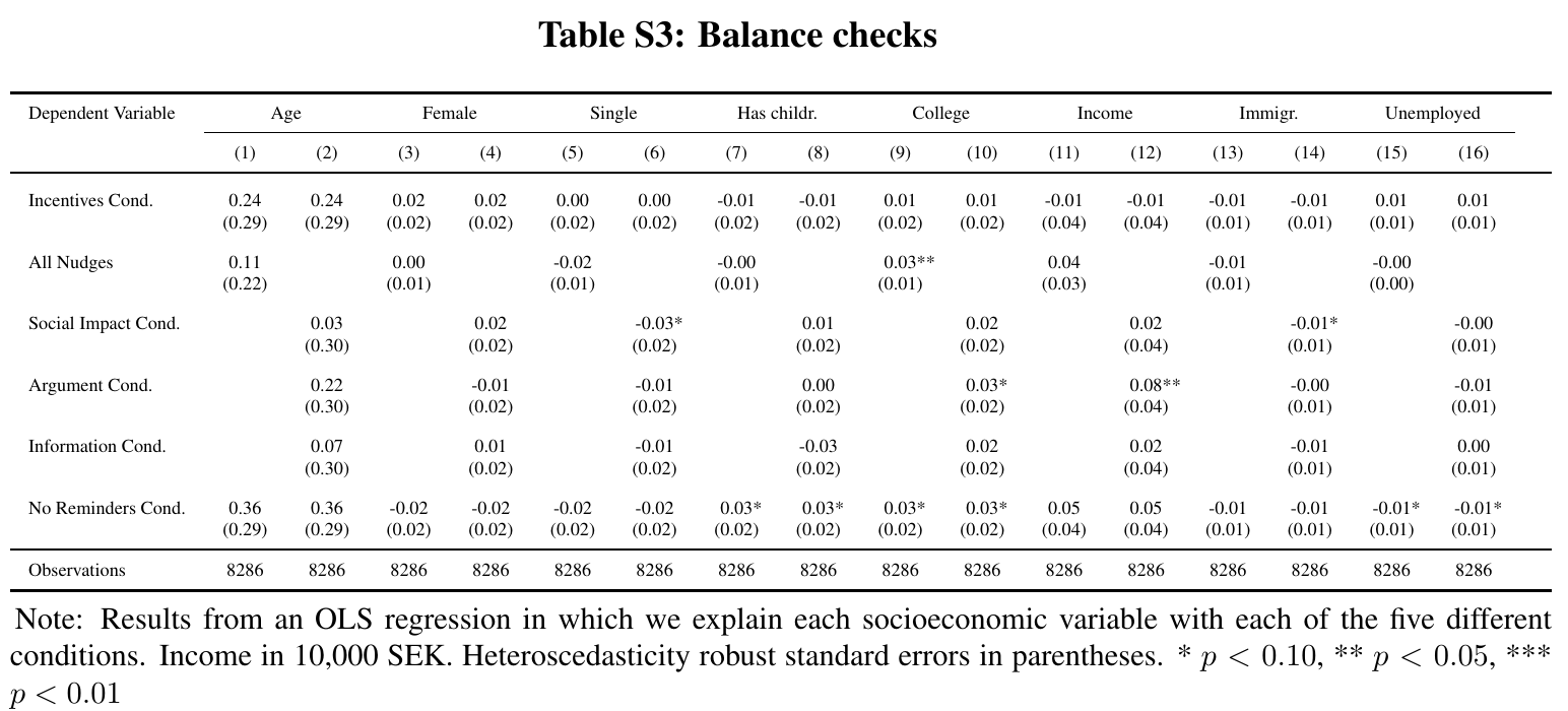
Campos-Mercade et al. (2021), supplementary Table S3, CC BY 4.0. Full-size table and notes.

Each baseline characteristic is regressed on assignment indicators. The coefficients are baseline differences, not effects on pre-existing characteristics. Intentions measured after assignment are not baseline characteristics.

Assignment and the Analysis Sample

The intervention is the offer of a payment, and vaccination is the outcome. Comparing people who actually received money with those who did not would select on the behaviour the intervention was intended to change.

In this application, examine survey completion, exclusion rules, and linkage to administrative records. Having an administrative outcome does not make the construction of the analysis sample irrelevant.

Intentions versus Behaviour

An intervention might change what people say they intend to do without changing what they actually do. The study observes both a survey response and subsequent vaccination in administrative records.

These are distinct outcomes. Their timing and measurement matter for interpreting the effects and their policy relevance.

Intentions were measured after assignment. They may themselves respond to the intervention, so they are not a baseline balance variable. Controlling for them in the uptake equation would change the total-effect question.

As you read the figures, identify the outcome, reference group, units, and confidence level before interpreting the estimate.

Figure 1

Figure 1

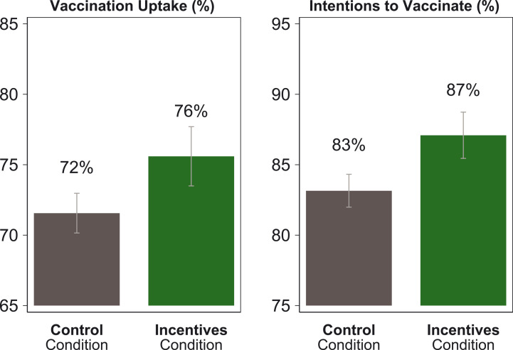
Campos-Mercade et al. (2021), Figure 1, CC BY 4.0. Bars show means; error bars are 90% confidence intervals.

Ask the assigned group to explain both panels, units, comparison group, and confidence intervals. These are raw group means. Figure 2 presents adjusted effects.

Figure 2

Figure 2

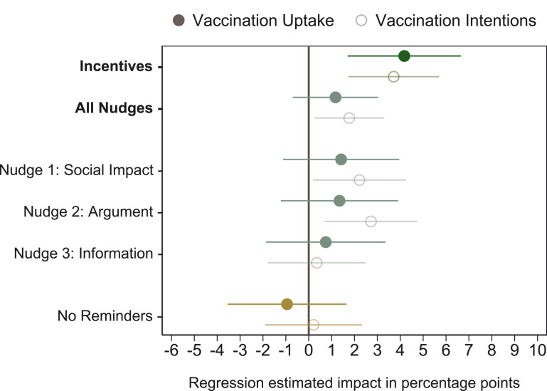
Campos-Mercade et al. (2021), Figure 2, CC BY 4.0. Adjusted effects; error bars are 90% confidence intervals.

Filled circles are uptake; open circles are intentions. Draw attention to the 90% intervals, which differ from default 95% intervals in Python output. Do not infer a difference between interventions solely from separate significance tests.

Interpreting the Results

Interpreting the Results

The adjusted payment effect on uptake is about 4.2 percentage points, against a control uptake rate of about 71.6%. The raw difference in Figure 1 is about 4.0 points; Figure 2 adjusts for baseline characteristics.

An effect in percentage points is a difference in probabilities. A relative percentage change divides that difference by the control probability.

Some nudges affect intentions more clearly than uptake. An insignificant coefficient does not establish a zero effect, and “significant here, insignificant there” is not itself a test that two effects differ.

The policy judgement also depends on costs, who responds, and whether the effect persists or generalises.

Spillovers

In vaccination, other people’s vaccination can affect exposure to infection; participants could also influence one another’s decision to vaccinate.

Distinguish the effect of a payment offer on vaccination uptake from vaccination’s effect on infection risk. The latter has an obvious spillover channel; interference must be considered in relation to the particular treatment and outcome.

External Validity

External Validity

The policy effect may vary with who receives treatment and how the programme is delivered. Differences in sample composition matter especially when effects differ along those characteristics.

Consider:

• A different age distribution, education mix, or immigration background.
• Another payment amount or an offer made by a government rather than researchers.
• Another country, level of trust, or stage of the vaccination rollout.

Table S3 compares the experimental arms. Table S4 compares the sample with the Swedish population aged 18–49. Neither table substitutes for the other.

Read Table S4’s footnotes as well as its means: some population measures are not defined identically. Similar observable characteristics alone cannot establish that the effect will travel.

After class: replicate and explain

• Construct the pooled nudge indicator.
• Replicate Table S3 and Table S5.
• Comment on Table S4, including its footnotes.
• Compare default and HC1 standard errors.
• Explain why outcome coefficients differ in scale from the paper.

Ungraded. Code and short interpretations in Quarto.

Textbook references

• The Effect: Chapters 6-8, 10, and 13.
• Causal Inference: The Remix: Chapters 3 and 4.
• Mastering ’Metrics: Chapters 1 and 2.
• Optional advanced: Mostly Harmless Econometrics: Chapters 2 and 3.

Reading guide and links

Sources and materials

Week 1 notes · Exercise

Supplement · Trial and PAP · Data

References

• Allcott, H. (2015). “Site Selection Bias in Program Evaluation.” Quarterly Journal of Economics 130(3): 1117–1165.

• Campos-Mercade, P., A. N. Meier, F. H. Schneider, S. Meier, D. Pope, and E. Wengström (2021). “Monetary incentives increase COVID-19 vaccinations.” Science 374(6569): 879–882.

• Freedman, D. A. (2008). “On regression adjustments to experimental data.” Advances in Applied Mathematics 40(2): 180–193.

• Harrison, G. W., and J. A. List (2004). “Field Experiments.” Journal of Economic Literature 42(4): 1009–1055.

• Lee, D. S. (2009). “Training, Wages, and Sample Selection: Estimating Sharp Bounds on Treatment Effects.” Review of Economic Studies 76(3): 1071–1102. (Link to author manuscript.)

• Lin, W. (2013). “Agnostic notes on regression adjustments to experimental data: Reexamining Freedman’s critique.” Annals of Applied Statistics 7(1): 295–318.

• Vivalt, E. (2020). “How Much Can We Generalize From Impact Evaluations?” Journal of the European Economic Association 18(6): 3045–3089.